
| Cerius2 Modeling Environment |
This section explains
This section tells you how to accomplish:
The basics of starting Cerius2 and using its interface are demonstrated in Introducing Cerius2 and described in The Cerius2 Interface.
You need to know how to build (Basic building) and/or load (Loading model structure files) a model and should know how to select atoms in your model (Selecting atoms and groups of atoms).
If your session contains several models, you should know how to specify the current model (Specifying the current model). You may also want to know how to select atoms in several models (Selecting atoms in several models).
Changing the position, viewing angle, and magnification of models in the model window aid in tasks such as accessing parts of the model, viewing small parts of the model in detail, understanding the model's 3D structure, bringing related or complementary models together in space, optimizing displays for printout.![]()
Moving models on the screen
This section includes information on:
Related information
Moving parts of models is discussed under Editing the structure. Copying models or parts of models from one model space to another is discussed under Moving models between model spaces.
Basic tasks and methods
Basic model-viewing tasks can often be accomplished in several ways: by using the mouse in the model window, using tools in the toolbar of the Cerius2·Visualizer's main control panel, using control panels accessed from menu items in the main control panel (mainly from the View menu), or using keyboard shortcuts. The various methods differ in convenience, quickness, and/or accuracy.
| The basic model viewing tools do not alter the original coordinates of the models. They affect only the view and appearance of models in the model window. |
Basic model-viewing tasks affect all models and include:
Display axes
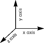
You rotate and translate models relative to the x, y, and z display (window) axes, which are always oriented as shown in Figure 3. (These window axes are not the same as the model's viewing-angle axes, which are usually displayed in the lower right corner of the model window, see Default annotation.)
|
A tutorial example of basic model moving is found in Moving a model.
Translating models
Manual translation
To interactively translate models, place the cursor in the model window and then press the middle mouse button and drag the mouse in any direction within the xy plane.
Select the View/Dials... menu item to access the Viewing Dials control panel.
Please see the on-screen help for details on the functioning of each control in the Viewing Dials control panel. Mouse functions and keyboard shortcuts are summarized in Mouse and Keyboard Actions.
Rotating models
Manual rotation
To interactively change the viewing angle of models, place the cursor in the model window and then:
| The default mouse behavior described here can be altered by changing the mouse rotation action from normal to continuous or rock (see Changing the default mouse rotation action). |
Changing the default mouse rotation action
To quickly change the viewing angle in large steps, place the cursor in the model window and then:
Select the View/Dials... menu item to access the Viewing Dials control panel.
Select the View/Dials... menu item to access the Viewing Dials control panel.
You can orient the view so that selected atoms in the current model lie parallel or perpendicular to the computer screen.
Please see the on-screen help for details on the functioning of each control in the Viewing Dials, Orient View, and View Options control panels. Mouse functions and keyboard shortcuts are summarized in Mouse and Keyboard Actions.
Changing the view magnification
Manual zooming
Filling the model window
To obtain the largest viewing area possible, you can change the size of the model window.
To return the model window to its usual size, you can:
Select the View/Dials... menu item to access the Viewing Dials control panel.
Select the View/Dials... menu item to access the Viewing Dials control panel.
Please see the on-screen help for details on the functioning of each control mentioned here. Mouse functions and keyboard shortcuts are summarized in Mouse and Keyboard Actions.
Setting position and orientation
Topics in this section include: resetting the view of the models to the default position, orientation, and magnification; centering the display (the differences between centering and resetting are presented in this section); and defining a center of rotation for the current model.
Resetting changes the viewing angle so that the model's x, y, and z axes are coincident with the window x, y, and z axes. Any translations are reversed by returning the model to the origin, and the magnification is returned to unity.
![]()
Centering a model translates it so that its center of rotation is in the center of the screen. Centering does not change the viewing angle or magnification. Centering immediately after defining the center of rotation (see Defining the center of rotation) affects only the current model. Centering after some other change in the model view moves all models in concert.
To center the model(s), you can do any of:
Please see the on-screen help for details on the functioning of each control mentioned here. Mouse functions and keyboard shortcuts are summarized in Mouse and Keyboard Actions.
Moving models relative to one another
You can move one model relative to another, for example, to investigate how a ligand fits in a receptor site.
Select the Move/Model Move... menu item to access the Model Space Transforms dcontrol panel. The current model is the one that is rotated and/or translated.
Simply make the desired models visible (Controlling model visibility and the display mode). Using the overlay display mode (Controlling model visibility and the display mode) and hiding any models you are not currently working with (Controlling model visibility and the display mode) should be most convenient; however, any display mode may be used.
Use any of the conventional means of defining a model as current (Specifying the current model).
To translate the current model, you can:
You can define a translation direction by entering a value in the Translate/Rotate Axis entry box or selecting some atoms and then clicking the associated DEFINE pushbutton in the Model Space Transforms control panel.
The rotation axes are the display axes, as shown in Figure 3.
To rotate the current model, you can:
You can define the center of rotation and rotation axis by entering values in the Rotation Center and Translate/Rotate Axis entry boxes or selecting some atoms and then clicking the associated DEFINE pushbuttons in the Model Space Transforms control panel.
When you save the model in .msi format (Saving model structure files), both its original coordinates and the transform for generating the transformed coordinates are automatically saved.
Please see the on-screen help for details on the functioning of each control in the Model Space Transforms control panel. Mouse functions and keyboard shortcuts are summarized in Mouse and Keyboard Actions.
Superimposing models
You can superimpose (or "match") models by performing a least-squares fit between selected atoms. Whole (nonperiodic) models or the asymmetric unit of periodic models can be superimposed. One model is translated and rotated as a rigid unit to obtain the best rms fit of the selected atoms with those of a reference (or target) model. This is useful for comparing structures of all or parts of models.
Select the Move/Atoms Match... menu item to access the Match Models control panel.
Specify which model is the reference model and which is the movable model by selecting them from the pulldowns or typing their model numbers or names in the text entry boxes.
The number of atoms specified in the reference model must be the same as the number in the moving model.
If you want or need to select the atoms to be matched, select them in the same order in both models. If atoms in the two models are numbered identically and you want to superimpose identically numbered atoms, you need select atoms only in one model.
You can mass-weight the calculation (for example, if the positions of hydrogens are less important) by setting the atom weighting popup to MASS.
Please see the on-screen help for details on the functioning of each control in the Match Atoms control panel. Selecting atoms in more than one model is discussed in Selecting atoms in several models.
The Cerius2·Align Molecules module (which is separately licensed and documented and is typically found in the DRUG DISCOVERY deck of cards) offers additional functionality for comparison of model structures.
Storing and retrieving views
You can save the current view (that is, the model and its viewing conditions such as orientation, location, magnification) in memory for later retrieval during the current session. Up to ten views can be saved and retrieved for later viewing within the current session.
To store a view, select the View/Orient... menu item to access the Orient View control panel. Set the View A-J popup as desired and click the STORE pushbutton.
To retrieve a view, select the View/Orient... menu item to access the Orient View control panel. Choose the desired view from the View A-J popup and click the RETRIEVE pushbutton.
Please see the on-screen help for details on the functioning of each control in the Orient View control panel.
The Visualizer animation facilities enable you to create an animation sequence from a trajectory file (such as that produced by the Cerius2·Dynamics Simulation module), and then replay that sequence using VCR-style controls.![]()
Animating models
How to produce trajectory files is discussed in the documentation for the relevant application modules (which are purchased separately).
Animating a model is a three-stage process. You first need to select a trajectory (.trj) file and load the information from it. Next you build an animation sequence. (Alternatively, check the Automate Build check box before loading the file.) Finally, the model is animated by "playing back" the animation sequence.
Select the View/Animation... menu item (on the main control panel's menu bar) to access the Animation control panel.
Use the file browser and selector tools to choose the trajectory file from which to construct the animation sequence. How to use these tools is detailed under Loading model structure files. (All file browsers work similarly.)
If the trajectory file you request appears to be associated with the current model, Cerius2 asks if you want to use this model as the initial frame of the trajectory. Otherwise, Cerius2 loads the associated MSI-format model file as the current model.
To build an animation sequence that uses all frames from a trajectory file, simply check the Automate Build check box before selecting the trajectory file.
Once the desired frames have been built into an animation sequence, you can use the Replay Animation controls to animate the model by replaying all or specified frames. These controls operate similarly to those on a tape recorder or VCR.
Animation sequences consume a considerable amount of memory. When you have finished with a sequence, you should clear the memory buffer in which it is held, by clicking the Clear All Frames action button in the Animation control panel.
Please see the on-screen help for details on the functioning of each control in the Animation and Frame Filter control panels.
Why read this section
![]()
Labeling and annotating models
Cerius2 allows you to label atoms according to various properties such as element names, atom type, charge, temperature, hybridization, etc. You can also annotate models by adding text and graphical objects such as arrows and boxes. In addition, the default type of annotation that Cerius2 always shows in the model window can be changed.
This section includes information on:
Related information
You can also enhance model displays by, for example, coloring atoms according to various properties (Model display colors) or color-mapping properties onto model surfaces (in, for example, the quantum chemical application modules, which have separate documentation).
Labels
Labels can be applied to entire models (when all or no atoms are selected) or to selected atoms within one or more models. Different labels may be used for different parts of a model.
NO LABEL
No labels
NUMBERS
Atom serial numbers
SYM/NUM
Crystal symmetry copy plus atom serial numbers
ELEMENTS
Element types
CHARGES
Atom partial charges
FORMAL CHARGE
Atom formal charges
OCCUPANCY
Atom site occupancies
ISOTROPIC
Atom isotropic temperature factors
FFYTPE
Forcefield atom types
HYBRID
Atom hybridization
NAME
Atom name
MASS
Atom mass
CHIRALITY
Atom chirality
To add, change, or remove labels on all or selected atoms, you can:
| You can interactively query the current properties of an atom by shift-clicking the atom with the right mouse button. A message box appears that lists the coordinates and properties of the atom. |
Bonds can be labelled with their fractional bond orders.
A tutorial example of labeling a model is found in Labeling a model.
Please see the on-screen help for details on the functioning of each control in the Display Attributes control panel and in the toolbar.
Measuring distances, angles, planes, torsions, and inversions for the atoms in a model and displaying these measurements in the model window is discussed under Measuring models.
Default annotation
Basic information that is usually shown by default comprises the model name and model space number (in the lower left corner of the model window) and a small set of axes indicating the viewing angle (lower right corner). You may hide this information if you prefer.
To change the default information shown in the model window, select the View/Options... menu item to access the View Options control panel. Check or uncheck the appropriate View Annotation check boxes.
Please see the on-screen help for details on the functioning of each control in the View Options control panel.
Custom annotations
Accessing the annotation
tools
Select the Build/Annotation... menu item to access the Annotation control panel.
The Annotation control panel contains several types of tools to help you highlight and enhance your displayed model:
![]()
![]()
![]()
![]()
![]()
Editing the annotation objects
You can use the annotation tools discussed in this section in two ways:
To specify that rectangles or circles be drawn in filled or outline style, check or uncheck the Filled check box. The fill color is always the same as the outline color.
You can move, change the size of, delete, or hide annotation objects:
![]()
An UNDO pushbutton, provided at the top of the control panel, can be used to cancel one or a series of previous commands for many types of operations. The UNDO button is greyed out when there is nothing to cancel.
Checking the Guide? check box gives you on-screen help (in the upper left corner of the model window) on the Annotation control panel functions.
Please see the on-screen help for details on the functioning of each control in the Annotation control panel.
Why read this section
![]()
Model display style
You can change the model display to suit your needs. For example, you may want to display molecules in traditional stick style or with ellipsoids representing thermal movements of atoms, you may want to emphasize some atoms, or you may want to view a cross section of a model.
This section includes information on:
Related information
Labeling atoms according to various properties is discussed under Labels. Setting the graphical quality and screen resolution is discussed under Resolution and graphical quality.
You can also enhance model displays by, for example, coloring atoms according to various properties (Model display colors) or adding Connolly (Model surfaces) or other surfaces.
Atom and bond display styles
Display styles can be applied to entire models (when all or no atoms are selected) or to selected atoms within one or more models. Different display styles may be used for different parts of a model.
This section includes information on displaying:
Example
A tutorial example of changing model display styles is found under Changing the display style.
Please see the on-screen help for details on the functioning of each control mentioned in this section.
Bonds as sticks
Understanding the display
The default is to display bonds as single, double, or triple lines. Atoms are not specifically shown, but are present at the ends of bonds. The bond colors represent the element types of the atoms at each end.

To reset stick display style, you can:
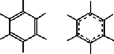
Multiple bonds can be shown as a set of parallel lines representing the bond order. Partial-double bonds in 6-membered ring systems can be represented as (both displayed and stored with the model as) Kekule or resonant bonds (Figure 4).
|
In addition, all bonds can be displayed as single lines regardless of the bond order (and without changing the actual bond order). This is useful, for example, for simplifying the display when viewing large models at small magnification. It does not change the actual bond type, which is stored with the model.
To display all bonds (in all models) as single lines (regardless of actual bond type), select the View/Display Attributes... menu item to access the Display Attributes control panel. Click the Preferences... pushbutton to access the Style Preferences control panel. Uncheck the Highlight Multiple Bonds check box.
Bonds as cylinders
Understanding the display
Cylinder style is similar to stick style, except that the bonds are represented by cylinders, providing a more three-dimensional representation. Atoms are not specifically shown, but are present at the ends of bonds. The bond colors represent the element types of the atoms at each end.

To display bonds in cylinder style, you can:
To set the radius of the cylinders, click the Preferences... button in the Display Attributes control panel to access the Style Preferences control panel. Enter the desired radius in the Cylinder Radius entry box.
Lone atoms
Understanding the display
Lone (not bonded) atoms in a model can be represented as three-dimensional crosses, small spheres, or simple points or can be not displayed at all.
To change how lone atoms are displayed, select the View/Display Attributes... menu item to access the Display Attributes control panel. Click the Preferences... button to access the Style Preferences control panel. In the latter control panel, set Lone Atom Style to CROSS, BALL, POINT, or NONE.
Atoms as balls
Understanding the display
Atoms can be represented by space-filling balls. If any bonds are visible between balls, they are represented as lines.

To display atoms in ball style, you can:
The ball radii are proportional to the van der Waals radius of the respective atoms. To set the ratio of ball radius to van der Waals radius, click the Preferences... pushbutton in the Display Attributes control panel to access the Style Preferences control panel. Enter the desired proportion in the Ball: Ball Size entry box.
Ball and stick models
Understanding the display
Ball and stick style represents atoms as van der Waals spheres and by bonds as cylinders.

To display models in ball and stick style, you can:
The ball radii are proportional to the van der Waals radius of the respective atoms. To set the ratio of ball radius to van der Waals radius, click the Preferences... pushbutton in the Display Attributes control panel to access the Style Preferences control panel. Enter the desired proportion in the Ball & Stick: Ball Size entry box.
To set the radius of the sticks, click the Preferences... button in the Display Attributes control panel to access the Style Preferences control panel. Enter the desired radius in the Stick Radius entry box.
Cations as polyhedra
Understanding the display
Polyhedra are used to simplify structural display for inorganic systems that contain tetrahedrally, octahedrally, or square- planar coordinated units, for example, zeolites, the high Tc superconductors, and multi-molybdates.
To display cations as polyhedra, you can:
Other atoms (non-cations) can be represented as crosses, small spheres, or single pixels or not drawn at all. To change how other atoms are displayed, click the Preferences... button in the Display Attributes control panel to access the Style Preferences control panel. Then set Non-Polyhedral Style to CROSS, BALL, POINT, or NONE.
Thermal ellipsoids
Understanding the display
Ellipsoid style represents a constant-probability surface for the thermal motion of the atoms. Atoms described by anisotropic temperature factors are represented by ellipsoids. (Atoms described by isotropic temperature factors are represented by spheres.) Lines representing bonds are drawn by default but can be removed. The orientation of the ellipsoid's principal axis may be displayed.
To display atoms as thermal ellipsoids, you must first be sure that anisotropic temperature factors (see Understanding the display and Temperature factors) have been specified or loaded. Then you can:
To show or hide the principal ellipsoid axis, click the Preferences... pushbutton in the Display Attributes control panel to access the Style Preferences control panel. Check or uncheck the Show Principal Axes check box.
You can define a scaling factor for the display size of thermal ellipsoids. A value of 1.0 corresponds to an ellipsoid whose radius at any point on the surface is equal to the root mean square (rms) atomic vibration in that direction. At a scaling factor of 1.0, the probability of the atom actually lying within the ellipsoid is low. Greater values produce greater probabilities, as shown in Table 7.
| Scale factor | Probability of atom being within ellipsoid |
|---|---|
| 1.54 | 50% |
| 2.02 | 75% |
| 2.50 (default) | 90% |
| 2.80 | 95% |
| 3.37 | 99% |
To set the scale factor for thermal ellipsoids, select the View/Display Attributes... menu item to access the Display Attributes control panel. Click the Preferences... pushbutton in the Display Attributes control panel to access the Style Preferences control panel. Enter the desired scale factor in the Ellipsoid Size entry box.
Structure traces
You can make only a structural trace of a model visible. This is done differently, depending on whether the model is a protein or any other kind of polymer.
To display only the backbone atoms of a polymer, select the View/Atom Visibility... menu item to access the Atom Visibility control panel. Click the Hide Non-Backbone Atoms action button. You must have previously defined some atoms as backbone atoms, using the Polymer Builder tools.
![]() -carbon trace of proteins
-carbon trace of proteins
To display an alpha carbon trace of a protein model:
Please see the on-screen help for details on the functioning of each control in the Atom Visibility and Display Attributes control panels.
Cross sections of models
You can control the apparent location of the viewing plane along a line perpendicular to the computer screen, as well as the plane's thickness, so as to view either the whole model or a cross section (slice or slab) through it. You do this by clipping the view between two coordinates of the screen z axis (that is, to set the apparent distance of the viewing plane from the computer screen).
Please see the on-screen help for details on the functioning of each control in the Z-Clipping control panel.
Apparent depth effects
Depth cueing
Depth cueing gives models an appearance of depth by displaying objects that are apparently closer to the surface of the computer screen in true color and mixing the color with the background color for objects that appear to be farther behind the surface of the computer screen. The extent of depth cueing can be changed.
Select the View/Graphics/Depth Cueing... menu item to access the Depth Cueing control panel.
To adjust the degree of depth cueing, use the Depth Cue Factor slider or its associated entry box. A value of 1 means that apparently near and far objects are all drawn with full color intensity; a value of 0 means that far objects disappear into the background.
Please see the on-screen help for details on the functioning of each control in the Depth Cueing control panel.
Projection
The projection method is another way of enhancing the appearance of depth in models. Two methods are available:
Select the View/Graphics/Projection... menu item to access the Projection control panel.
Choose the desired projection method from the control panel. If you choose PERSPECTIVE, you can specify the projection angle by entering a number in the Angle entry box.
Please see the on-screen help for details on the functioning of each control in the Projection control panel.
Object resolution
![]()
Resolution and graphical quality
The balls, ellipsoids, and cylinders produced by the various display styles are represented on-screen as multifaceted polyhedral facets (for balls and ellipsoids) and prismoidal facets (for cylinders). A small number of facets used to draw an object results in a fast but coarse display. Large numbers of facets improve smoothness and specularity, but at the expense of drawing speed. The default value usually provides a reasonable compromise between display speed and resolution.
To change the line width used to draw (non-cylinder) bonds, select the View/Display Attributes... menu item to access the Display Attributes control panel. Click the Preferences... pushbutton to access the Style Preferences control panel. Adjust the Line Width slider by dragging or directly enter values in the associated entry box.
Cerius2 enables you to specify the quality of graphics displayed on the computer and written to vector PostScript files. Three quality settings are available: standard, better, and excellent. Higher quality settings reduce the golf-ball effect that results because X and vector PostScript triangles are flat-shaded instead of color-interpolated. However, each higher quality setting can also increase both the file size and the rendering time by a factor of four over the previous quality setting.
To adjust the graphics quality, select the View/Display Attributes... menu item, then click the Preferences... button in the Display Attributes control panel. In the Style Preferences control panel that appears, set X/PostScript Quality to STANDARD, BETTER, or EXCELLENT. Each higher quality setting can increase both the file size and the rendering time by a factor of four over the next-lower quality setting.
Please see the on-screen help for details on the functioning of each control in the Style Preferences control panel.
Why read this section
![]()
Printing models and graphs
This section includes information on:
Setting the print resolution is discussed in Resolution and graphical quality. Using PSYCHO within Cerius2 for rendering models (and producing PostScript output) is discussed in Rendering and ray-tracing.
You need to know what UNIX print command (including command-line options) is usually used at your site for sending PostScript output from applications to a printer. Please ask an experienced user at your site, or your system administrator, if you do not know the command.
Select the File/Print... menu item to access the Print control panel. This contains the primary PostScript output controls and provides access to the Page Setup control panel, which contains supplementary controls.
Select the image source by setting Image Capture to Model Window or Graph Window. The size of the model window affects the image's detail when it is output as bitmap PostScript: the larger the window, the greater the detail. However, the size of the graph window does not affect the output detail.
You can access some less frequently used controls by clicking the Page Setup... pushbutton in the Print control panel, which causes the Page Setup control panel to appear.
If you are printing the image in the model window, you can choose to output in vector PostScript or screen dump (raster) format. Vector PostScript images are device-independent, can be resized without loss of display quality, and can produce better quality output (colors, shapes, and so on) on a PostScript printer. Raster images, such as screen dump images, may become distorted when they are scaled.
You can specify the resolution (in dots per inch) for curves in graphs. Increasing this value allows improved definition of these images, although the resolution of the output device is always a limiting factor. Increasing the resolution results increases the PostScript image generation time, file size, and printing time.
If you run Cerius2 on an SGI platform, you can click the PREVIEW pushbutton in the Print control panel. This calls up SGI's xpsview utility, to preview your PostScript image before sending it to the printer or a file.
Once all options have been set to your satisfaction, click the PRINT pushbutton in the Print control panel.
A tutorial example of printing a model is found under Printing a model.
Please see the on-screen help for details on the functioning of each control in the Print and Page Setup control panels. Changing the resolution with which graphics are displayed and written is covered under Resolution and graphical quality.