
| Quantum 1 Modules |
Commands are described in alphabetical order in this section. Frequently used keywords are listed according to function in DMol3--Keyword Reference.
The .input file is a simplified command input file that consists of keywords followed by values (real, integer, or character). These keywords and their values specify flags for the calculation, such as the type of basis set or the maximum number of self-consistent iterations to be employed.
The rest of this section contains detailed descriptions of each of the commands available in the standalone version. For each command, documentation is divided into subsections.![]()
Format for documenting DMol standalone commands
The Syntax subsection begins with the command syntax presented in as generic a form as possible. Several type style conventions are used to distinguish different kinds of words. For example:
Atom_Calculation
Purpose
The Atom_Calculation keyword indicates that an .inatom file is read in, so that a user-specified atomic basis set can be created.
Syntax
Atom_Calculation value
Description
The atomic calculations are performed using information in the .inatom file for the DFT functional as specified by Functional keyword. Atomic calculations can be relativistic if the Pseudopotential VPSR keyword is specified.
Atom_Rcut
Purpose
The Atom_Rcut keyword allows you to specify the use of real-space cutoffs in the calculation of atomic basis sets.
Syntax
Atom_Rcut value
| command keyword | values | default | meaning |
|---|---|---|---|
|
Atom_Rcut
|
real > 0
|
5.5
|
The basis set cutoff in angstroms.
|
Description
You can input Atom_Rcut in Bohrs by specifying:
Atom_Rcut real>0 AUFor Harris calculations, you may use an even smaller cutoff of 4.5 Å. A smaller cutoff improves computational performance but may diminish the accuracy of calculations.
Description
Aux_Density is used to specify the maximum angular momentum of the multipolar fitting functions that specify the analytical form of the charge density and the Coulombic potential.
By default, the Lmax for the hydrogen atom is 1 less than for all other atoms. You can input Lmax for every type of atom by using the user keyword.
Example
Consider Fe(C5H5)2. An Aux_Density specification of:
Aux_Density quadrupolemeans that up to l = 2 functions are used to fit the density of all atoms except H (for which l = 1).
If you want to use a different fitting accuracy for Fe, you can use the user option, for example:
Aux_Density userwhich tells the program to use up to l = 2 (quadrupole-type) functions on C, only dipole functions on H, and up to l = 3 functions on Fe.
6 2
1 1
26 3
The default specification is octupole, which corresponds to the following Lmax values:
Lmax 3 2 3and which tells the program to use up to l = 3 functions on C, quadrupole-type functions on H, and up to l = 3 functions on Fe.
|
The keyword for integration is Integration_Partition. |
| command keyword | values | default | meaning |
|---|---|---|---|
|
Aux_Partition
|
integer
|
11
|
Selects the partition function.
|
| 1
The value of this number = n, where n is shown as ng
|
Description
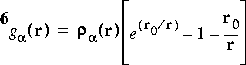
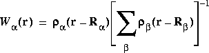
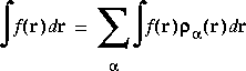
The value refers to the auxiliary partition function to use in the calculation. See Eq. 20 for the definition of a partition function.
The preferred choice for the auxiliary partition function is:
Eq. 2
![]() where r = |ri - R
where r = |ri - R![]() |, r0 = 0.5, and
|, r0 = 0.5, and ![]() a is the atomic charge density for atom
a is the atomic charge density for atom ![]() . This is function number 1.
. This is function number 1.
Eq. 3
![]()
Eq. 4
![]()
Eq. 5
![]()
Eq. 6
![]()
Eq. 7
![]()
Eq. 8
Eq. 9
![]()
Eq. 10
![]()
Eq. 11
![]()
Eq. 12
![]()
Eq. 13
![]()
Basis
Purpose
Basis allows you to specify the atomic basis set. This is the number and type of atomic orbitals used in the expansion of the molecular orbitals.
Syntax
Basis value_keyword
[value_number ...
blank line]
1
For example, the polarization function on H is 2p, on C is 3d, and on Fe is 4p.
Description
The size of the DND basis is comparable to Gaussian 6-31G* basis sets, and DNP basis sets are comparable to 6-31G** sets. However, the numerical basis set is much more accurate than a Gaussian basis set of the same size.
atomic_number nfrz nnls(i), i=1,nfrznfrz is the number of atomic basis functions on the atom, and nnls(i) tells DMol3 how to treat the ith function of the atom. nnls(i) = 0 means to include basis function +i in the calculation; and nnls(i) = 2 means to delete this basis function entirely.
Repeat atomic_number nfrz nnls(i), i=1,nfrz for each atom type, and terminate the list with a blank line.
As an example of mixed basis set input, consider the water molecule:
Basis mixedThis specifies a DNP basis set for oxygen and a DN basis set for hydrogen.
8 dnp
1 dn
<BLANK LINE>
Example 2
As an example of a user-specified basis set consider the following input and corresponding relevant parts of the output for an H2O molecule:
Basis dn
Output:
Specifications for basis set selection:The polarization functions have been eliminated from the basis set for both H and O.
Hydrogen nbas= 1 z= 1. 3 radial functions, spin energy= -0.033Ha
n=1 L=0 occ= 1.00 e= -0.233107Ha -6.3432eV
n=1 L=0 occ= 0.00 e= -0.845000Ha -22.9936eV
n=2 L=1 occ= 0.00 e= -2.000000Ha -54.4228eV eliminated
Oxygen nbas= 2 z= 8. 7 radial functions, spin energy= -0.054Ha
n=1 L=0 occ= 2.00 e= -18.758046Ha -510.4326eV
n=2 L=0 occ= 2.00 e= -0.871142Ha -23.7050eV
n=2 L=1 occ= 4.00 e= -0.338180Ha -9.2023eV
n=2 L=0 occ= 0.00 e= -2.130079Ha -57.9624eV
n=2 L=1 occ= 0.00 e= -1.593478Ha -43.3608eV
n=3 L=2 occ= 0.00 e= -2.722222Ha -74.0755eV eliminated
n=3 L=2 occ= 0.00 e= -1.388886Ha -37.7935eV eliminated
Input:
Basis userOutput:
8 7 0 0 0 0 0 2 0
Specifications for basis set selection:Here, the user redefined the oxygen basis set by selecting the second polarization function to be available for molecular calculations of H2O.
Hydrogen nbas= 1 z= 1. 3 radial functions, spin energy= -0.033Ha
n=1 L=0 occ= 1.00 e= -0.233107Ha -6.3432eV
n=1 L=0 occ= 0.00 e= -0.845000Ha -22.9936eV
n=2 L=1 occ= 0.00 e= -2.000000Ha -54.4228eV eliminated
Oxygen nbas= 2 z= 8. 7 radial functions, spin energy= -0.054Ha
n=1 L=0 occ= 2.00 e= -18.758046Ha -510.4326eV
n=2 L=0 occ= 2.00 e= -0.871142Ha -23.7050eV
n=2 L=1 occ= 4.00 e= -0.338180Ha -9.2023eV
n=2 L=0 occ= 0.00 e= -2.130079Ha -57.9624eV
n=2 L=1 occ= 0.00 e= -1.593478Ha -43.3608eV
n=3 L=2 occ= 0.00 e= -2.722222Ha -74.0755eV eliminated
n=3 L=2 occ= 0.00 e= -1.388886Ha -37.7935eV
Input:
Basis dnpOutput:
Specifications for basis set selection:An alternative input that leads to the same output is:
Hydrogen nbas= 1 z= 1. 3 radial functions, spin energy= -0.033Ha
n=1 L=0 occ= 1.00 e= -0.233107Ha -6.3432eV
n=1 L=0 occ= 0.00 e= -0.845000Ha -22.9936eV
n=2 L=1 occ= 0.00 e= -2.000000Ha -54.4228eV
Oxygen nbas= 2 z= 8. 7 radial functions, spin energy= -0.054Ha
n=1 L=0 occ= 2.00 e= -18.758046Ha -510.4326eV
n=2 L=0 occ= 2.00 e= -0.871142Ha -23.7050eV
n=2 L=1 occ= 4.00 e= -0.338180Ha -9.2023eV
n=2 L=0 occ= 0.00 e= -2.130079Ha -57.9624eV
n=2 L=1 occ= 0.00 e= -1.593478Ha -43.3608eV
n=3 L=2 occ= 0.00 e= -2.722222Ha -74.0755eV
n=3 L=2 occ= 0.00 e= -1.388886Ha -37.7935eV eliminated
Basis userFinally, you have complete control over the design of basis sets by specifying a run_name.inatom file. DMol3 creates an .inatm scratch file by default.
1 3 0 0 0
8 7 0 0 0 0 0 0 2
<BLANK LINE>
If the Atom_Calculation inatom keyword is specified, it overwrites the default design of orbitals. Instead, a run_name.inatm file is read and used to create atomic orbitals. The Basis keyword is still needed, since it serves to select which atomic orbitals are used in molecular calculations.
The contents and format of the .inatom file are documented below:
| 1
For hydrogenic orbitals (istart = -1), nprinc and lorb are hydrogenic functions to be included unchanged.
|
The following sample input and comments illustrate the use of the .inatom file in generating basis sets.
INPUT                      Comments
_____                      _________
1., 0, 0, 0, 0,            Normal run for hydrogen.
1., 0, 0, 1, 2,            Start with previous orbitals; compute spin energy.
1.3, 2, 0, -1, -1,         Generate hydrogenic orbitals with z = 1.3 for use as extended basis set;
                           orthogonalize to existing orbitals.
1, 0, 0., 0.,              Use a 1s hydrogenic orbital.
2, 1, 0., 0.,              Use a 2p hydrogenic orbital.

3., 0, 0, 0, 0,            Normal run for Li.
3., 0, 0, 1, 2,            Start with previous orbitals, compute spin energy.
3., 2, 0, 1, -1,           Start with previous orbitals; compute orbitals using new occupation to
                           be specified on next 2 lines; orthogonalize before writing out.
2, 0, -1., 0.,             Remove one alpha electron from 2s.
2, 1, 0., 0.               Use a 2p with unchanged occupation.

5., 3, 0, -1, -1,          Generate hydrogenic orbitals using Z = 5, for use as polarization and
                           extended functions.
3, 2, 0., 0.               Use 3d.
2, 1, 0., 0.,              Use 2p.
1, 0, 0., 0.,              Use 1s.
7., 3, 0, -1, -1,          Generate hydrogenic orbitals using Z = 7, for use as polarization and
                           extended functions.
3, 2, 0., 0.               Use 3d.
2, 1, 0., 0.,              Use 2p.
1, 0, 0., 0.,              Use 1s.

6., 0, 0, 0, 0,            Normal run for carbon.
6. 0, 0, 1, 2,             Start with previous orbitals, compute spin energy.
6., 1, 0, 1, -1            Start with previous orbitals; generate orbitals using new occupation
                           specified by 1 line (this will be C+2).
2, 1, -2., 0.              Remove 2 alpha electrons from 2p.
5., 3, 0, -1, -1,          Generate hydrogenic orbitals using Z = 5, for use as polarization and
                           extended functions.
3, 2, 0., 0.               Use 3d.
2, 1, 0., 0.,              Use 2p.
1, 0, 0., 0.,              Use 1s.
7., 3, 0, -1, -1,          Generate hydrogenic orbitals using Z = 7, for use as polarization and
                           extended functions.
3, 2, 0., 0.               Use 3d.
2, 1, 0., 0.,              Use 2p.
1, 0, 0., 0.,              Use 1s.

11., 0, 0, 0, 0,           Normal run for sodium.
11., 0, 0, 1, 2,           Start with previous orbitals, compute spin energy.
11., 4, 0, 1, -1           Start with previous orbitals; generate orbitals using new occupation
                           specified by next 4 lines; this will be Na+2 with extended functions.
2, 1, -1., 0.              Remove one alpha electron from 2p.
3, 0, -1., 0.,             Remove one alpha electron from 3s.
3, 1, 0. 0.,               Use 3p orbital, unoccupied.
3, 2, 0., 0.,              Use 3d orbital, unoccupied (polarization).

21., 0, 0, 0, 0,           Normal run for scandium.
21., 0, 0, 1, 2,           Compute spin energy.
21., 1, 0, 1, -1           Compute orbitals using new occupation defined by one line;
                           this will be Sc+2.
4, 0, -.1, -1.             Remove one alpha, one beta electron from 4s.
21., 2, 0, 1, -1,          Compute more orbitals using new occupation defined by next 2 lines;
                           this will be a 4s4p excited state.
4, 1, 1., 0.               Use 4p with 1 alpha electron added.
4, 0, -1., -1.             Use 4s with 1 alpha electron removed.

-1.                        End of input.
| command keyword | value keywords | default | meaning |
|---|---|---|---|
|
Basis_Version
|
default
|
default
|
Use basis set from the DMol 3.5 release.
|
|
|
v4.0.0
|
|
Use basis set from the DMol 400 release.
|
Description
This option allows for choosing a particular type of basis set. It is recommended that the v4.0.0 basis set be used for COSMO calculations, and the default be used for all other calculations.
Bond_Order
Purpose
The Bond_Order keyword allows for calculation of the Mulliken and Mayer bond orders and valence indices.
Syntax
Bond_Order value
| command keyword | value keywords | default | meaning |
|---|---|---|---|
|
Bond_Order
|
off
|
off
|
Do not calculate bond orders.
|
|
on
|
|
Do calculate bond orders.
|
Description
This option allows for useful analysis of bond and valence indices, which can be correlated with classical chemistry concepts of bond and reactivity.
Calculate
Purpose
The value of Calculate tells DMol which type of calculation you want to perform.
Syntax
Calculate value_keyword
Description and example
The Calculate keyword selects the type of calculation to perform. You provide one of the value keywords, for example:
Calculate frequency
| command keyword | values | default | meaning |
|---|---|---|---|
|
Charge
|
real
|
0.0
|
Total molecular charge of ionic systems.
|
Description
When Charge and Occupation Fermi are specified, DMol3 automatically chooses appropriate occupations for a neutral or ionic species.
COSMO
Purpose
The COSMO keyword is used to specify the COSMO solvation procedure.
Syntax
COSMO value
| command keyword | values | default | meaning |
|---|---|---|---|
|
COSMO
|
on
|
|
Perform COSMO calculations.
|
|
off
|
off
|
Do not use COSMO procedure.
|
Description
The COnductor-like Screening MOdel (COSMO) (Klamt and Schuurmann, 1993) is a continuum solvation model where the solute molecule forms a cavity within the dielectric continuum of permittivity ![]() that represents the solvent. The charge distribution of the solute polarizes the dielectric medium. The response of the dielectric medium is described by the generation of screening (or polarization) charges on the cavity surface.
that represents the solvent. The charge distribution of the solute polarizes the dielectric medium. The response of the dielectric medium is described by the generation of screening (or polarization) charges on the cavity surface.
The screening charges are determined from the boundary condition of vanishing potential on the surface of a conductor. COSMO provides the electrostatic contribution to the free energy of solvation. In addition there are nonelectrostatic contributions to the free energy of solvation which describe the dispersion interactions and cavity formation effects.
The DMol3/COSMO method has been tested extensively (Klamt et al. 1998). In order to improve accuracy, particularly for anions, the outlying charge correction was introduced (Klamt and Jonas, 1996). For further details, discussion of accuracy of the method and its extension, the user is encouraged to study the included references.
COSMO_RS
Purpose
The COSMO_RS keyword tells DMol3 to calculate macroscopic thermodynamic properties of solvents using the COSMO_RS model.
Syntax
COSMO_RS value
| command keyword | values | default | meaning |
|---|---|---|---|
|
COSMO_RS
|
on
|
|
Perform COSMO_RS calculations.
|
|
off
|
off
|
Do not use COSMO_RS procedure.
|
Description
The COSMO_RS model is an extension of the COSMO model beyond the dielectric approximation. Results of DMol3/COSMO calculations allow you to determine the chemical potential of the compound in the solvent, and consequently, properties of liquid/liquid and vapor/liquid systems such as vapor pressures or partition coefficients.
Since the COSMO_RS parameterization is somewhat dependent on the underlying DMol3/COSMO results it is recommended that you use the default parameters for the DMol3/COSMO/COSMO_RS run:
|
Functional
|
vwn-bp
|
|
basis
|
dnp
|
|
basis_version
|
v4.0.0
|
|
integration_grid
|
fine
|
|
atom_rcut
|
5.5
|
You can obtain detailed information from the COSMO_RS run and input the exact gas phase energy of the solute. The exact value of energy obtained from the separate calculations of the solute in the gas phase improves accuracy of the free energy of hydration and vapor pressure. To do this run DMol3/COSMO/COSMO_RS with the modified CRS_INPUT file present in the running directory. By default the CRS_INPUT file resides in the DMOL3_DATA directory.
Gas phase calculations must be performed at the same level of DMol3 as the DMol3/COSMO run.
COSMO_Dielectric
Purpose
The COSMO_Dielectric parameter specifies the dielectric constant of the solvent within the COSMO approach.
Syntax
COSMO_Dielectric value
| command keyword | values | default | meaning |
|---|---|---|---|
|
COSMO_Dielectric
|
real
|
999.9
|
This value corresponds to a conductor.
|
Description
The default value of 999.9 is appropriate for the COSMO_RS run. Any positive real value is within the range, e.g., water at room temperature has a dielectric constant of 78.4.
COSMO_Grid_Size
Purpose
The COSMO_Grid_Size parameter tells DMol3 how many basic grid points per atom to consider.
Syntax
COSMO_Grid_Size value
| command keyword | values | default | meaning |
|---|---|---|---|
|
COSMO_Grid_Size
|
integer
|
1082
|
Number of basic grid points.
|
Allowed values: 12, 32, 42, 92, 122, 162, 272, 362, 482, 642, 812, 1082, 1442, 1922.
Note
|
It is recommended that you use only the default value, i.e., 1082. |
Description
The COSMO surface surrounding the solute molecule is constructed as a superposition of spheres centered at the atoms, discarding all parts lying in the interior part of the surface. The spheres are represented by means of a discrete set of points, which is the so-called basic grid.
COSMO_Segments
Purpose
COSMO_Segments parameter specifies the maximum number of segments on each atomic surface.
Syntax
COSMO_Segments value
| command keyword | values | default | meaning |
|---|---|---|---|
|
COSMO_Segments
|
integer
|
92
|
Number of segments.
|
Allowed values: 12, 32, 42, 92, 122, 162, 272, 362, 482, 642, 812, 1082, 1442, 1922.
Description
The basic grid points (specified with the COSMO_Grid_Size parameter) are then assigned to segments, which also are represented as discrete points on the COSMO surface. The position of the screening charges equal the position of the segments.
COSMO_Solvent_Radius
Purpose
The COSMO_Solvent_Radius parameter specifies the solvent probe radius.
Syntax
COSMO_Solvent_Radius value
| command keyword | values | default | meaning |
|---|---|---|---|
|
COSMO_Solvent_Radius
|
real
|
1.3
|
Solvent probe radius.
|
Allowed values are between 0.5 and 2.0.
Note
This parameter is used in the construction of the COSMO cavity and should not be changed, especially when performing a COSMO_RS run.
COSMO_A-Matrix_Cutoff
Purpose
The COSMO_A-Matrix_Cutoff parameter determines the accuracy of the electrostatic interactions on the COSMO surface.
Syntax
COSMO_A-Matrix_Cutoff value
| command keyword | values | default | meaning |
|---|---|---|---|
|
COSMO_A-Matrix_Cutoff
|
real
|
7.0
|
A-Matrix_Cutoff threshold.
|
Note
The A-Matrix_Cutoff should not be smaller than 2.0.
Description
The calculation of the electrostatic interaction between surface charges is done based on either the segments or the basic grid, depending on the cutoff distance specified in COSMO_A-Matrix_Cutoff. If the distance between two segments is less than the cutoff value specified, the electrostatic interaction between segments is calculated using the basic grid. The basic grid method provides the higher accuracy required at shorter distances.
COSMO_Radius_Incr
Purpose
The COSMO_Radius_Incr parameter specifies the increment to the atomic radii used in the construction of the COSMO cavity.
Syntax
COSMO_Radius_Incr value
| command keyword | values | default | meaning |
|---|---|---|---|
|
COSMO_Radius_Incr
|
real
|
0.0
|
Increment of the atomic radii.
|
Note
This parameter is used in the construction of the COSMO cavity and should not be changed, especially when performing a COSMO_RS run.
COSMO_A-Constraint
COSMO_B-Constraint
Purpose
The COSMO_A-Constraint and COSMO_B-Constraint parameters are used to approximate the non-electrostatic contribution to the solvation energy within the COSMO model.
Syntax
COSMO_A-Constraint value
Description
The two parameters define the nonelectrostatic contribution via the equation:![]()
COSMO_RadCorr_Incr
Purpose
The COSMO_RadCorr_Incr parameter is used to construct the outer cavity for the outlying charge correction.
Syntax
COSMO_RadCorr_Incr value
| command keyword | values | default | meaning |
|---|---|---|---|
|
COSMO_RadCorr_Incr
|
real
|
0.15
|
Increase of the original cavity to evaluate outlying charge correction.
|
Note
This parameter is used in the construction of the COSMO cavity and should not be changed, especially when performing a COSMO_RS run.
Description
This is an important correction which accounts for the electron density leaking outside of the cavity boundary. It is of particular importance for anion calculations.
where:
Recommended radii are as follows:
| element | atomic number | radius |
|---|---|---|
|
H
|
1
|
1.30
|
|
C
|
6
|
2.0
|
|
N
|
7
|
1.83
|
|
O
|
8
|
1.72
|
|
Cl
|
17
|
2.05
|
Note
These parameters are used in the construction of the COSMO cavity. You must not use any other values when performing a COSMO_RS run.
Electric_Field
Purpose
The Electric_Field keyword specifies to impose a static electric field on the system (valid only for nonperiodic models).
Syntax
Electric_Field x_value y_value z_value
| command keyword | values | default | meaning |
|---|---|---|---|
|
Electric_Field
|
three reals
|
|
Electric field vector in atomic units.
|
|
off
|
off
|
Do not impose electric field.
|
Description
With this option, various properties can be studied in the presence of an electric field. In particular, the polarizability tensor can be computed by computing the dipole moment in the presence of electric fields in the x, y, and z directions.
Eq. 14
![]() In practice, these polarizability terms require at least four separate calculations: one without a field and one with the field in each of directions x, y, and z. More reliable results are obtained if fields are applied in both the positive and negative directions and the results are averaged.
In practice, these polarizability terms require at least four separate calculations: one without a field and one with the field in each of directions x, y, and z. More reliable results are obtained if fields are applied in both the positive and negative directions and the results are averaged.
Example
To impose an electric field of strength 0.001 atomic units in the y direction, enter:
Electric_Field 0.00 0.001 0.00
| command keyword | value keywords | default | meaning |
|---|---|---|---|
|
Electrostatic_Moments
|
off
|
off
|
Do not compute dipole moments.
|
|
on
|
|
Compute dipole moments.
|
Description
Dipole moments are printed in both atomic units and Debyes.
Functional
Purpose
The Functional keyword specifies the local correlation and gradient-corrected functionals for exchange and correlation.
Syntax
Functional value_keyword
Description
The extension of the Hedin-Lundqvist functional to spin-polarized systems is the von Barth-Hedin functional. DMol3 does not use the original BH parameters, instead using the ones used by Janak, Moruzzi, and Williams (JMW) from their original work on metals.
Functional_Post_LDA
Purpose
The Functional_Post_LDA keyword allows for calculation of the energy using a gradient-corrected functional at the end of the calculation.
Syntax
Functional_Post_LDA value_keyword
Description
A typical use of this command would be to carry out a geometry optimization at the local DFT level, followed by calculation of nonlocal DFT energies using the local DFT-optimized structure.
Grid
Purpose
The Grid keyword specifies the grid on which the electronic properties specified by Plot are evaluated.
Syntax
Grid value_keyword
[value_number ...]
| command keyword | value keywords | default | meaning |
|---|---|---|---|
|
Grid
|
box
|
box
|
Specify a rectangular grid around the molecule, on the next line.
|
|
user
|
|
Select a set of grid points in a more versatile way.
|
Description
The grid specified by Grid is different from the mesh used for numerical integration. Grid data are read only when Plot is used.
If the box option is used, the next line must contain the data (in free format):
ndim nx ny nz extndwhere:
       Grid   box
        3      5      5      5      10.0
Example 2
       Grid box
        3    -20      -20    -20     5
This is a very dense grid, which produces very large files.
| command keyword | value keywords | default | meaning |
|---|---|---|---|
|
Harris
|
off
|
off
|
Do not use Harris functional.
|
|
on
|
|
Use Harris functional.
|
Hirshfeld_Analysis
Purpose
The Hirshfeld_Analysis keyword specifies atomic population analysis by the Hirshfeld partitioning procedure.
Syntax
Hirshfeld_Analysis value ...
Description
The Hirshfeld partitioned charges are defined relative to the deformation density. The deformation density is the difference between the molecular and the unrelaxed atomic charge densities and is given by:
Eq. 15
 where
where ![]() (r) is the molecular charge density and
(r) is the molecular charge density and ![]() a(r - R
a(r - R![]() ) is the density of the free atom
) is the density of the free atom ![]() at coordinates R
at coordinates R![]() . Using the deformation density, the effective atomic charges, dipoles, and quadrupoles on atom
. Using the deformation density, the effective atomic charges, dipoles, and quadrupoles on atom ![]() are defined as (Delley 1990):
are defined as (Delley 1990):
Eq. 16
![]()
Eq. 17
![]()
Eq. 18
![]() The weight W
The weight W![]() (r) is defined as the fraction of the atomic density from atom
(r) is defined as the fraction of the atomic density from atom ![]() at coordinate r:
at coordinate r:
Eq. 19
Integration_Grid
Purpose
The Integration_Grid keyword controls the selection of mesh points for the numerical integration procedure used in the evaluation of the matrix elements. Since the functions in these equations are given numerically, the choice of mesh points can have a significant impact on the final results.
Syntax
Integration_Grid value_keyword
[value_number ...
blank line]
Description
A value of medium appears to give a reasonable compromise between computational expense and numerical precision.
Radial points are taken in shells from the nucleus out to a distance of rmaxp (default = 10.0 au). The number of shells is a function of the nuclear charge, so that heavier elements have a greater number of points. The actual number is 14 X (Z + 2)1/3, where Z is the atomic number. The value of sp may be used to increase or decrease this number, that is, sp = 2.0 results in twice as many radial points.
Angular sampling points are generated on each shell using a spherical harmonic function. The initial number of angular sampling points is 14, generated with a harmonic function with l = 5. The number of angular points must be increased at larger radii in order to maintain the quality of the numerical integration. The value of thres specifies the requested numerical precision (default = 0.0001), and the number of angular points is increased to maintain the precision. The minimum value of the harmonic generator is given by iomin (default = 1) and the maximum allowed value by iomax (default = 4). The value cannot increase beyond iomax, even if numerical precision is compromised.
The following table gives the angular momentum of the spherical harmonic function used to generate the points on a radial shell and the number of such points:
| iomin (or iomax) | l | # points |
|---|---|---|
|
1
|
5
|
14
|
|
2
|
7
|
26
|
|
3
|
11
|
50
|
|
4
|
17
|
110
|
|
5
|
23
|
194
|
|
6
|
29
|
302
|
|
7
|
35
|
434
|
|
8
|
41
|
590
|
The value of ipa (default = 6) controls the partition function used to improve the convergence of the numerical integration.
| Integration_Grid value | ipa | iomax | iomin | thres | rmaxp | sp |
|---|---|---|---|---|---|---|
|
xcoarse
|
6
|
3
|
1
|
0.01
|
10.0
|
1.0
|
|
coarse
|
6
|
4
|
1
|
0.001
|
10.0
|
1.0
|
|
medium
|
6
|
6
|
1
|
0.0001
|
10.0
|
1.0
|
|
fine
|
6
|
6
|
1
|
0.00001
|
12.0
|
1.2
|
|
xfine
|
6
|
7
|
1
|
0.000001
|
15.0
|
1.5
|
To input values for these six parameters via the user option, begin immediately after the keyword Integration_Grid line and enter the data for npri, iomax, iomin, thres, rmaxp, and sp on a single line. (npri > 0 results in the printing of debug information.)
Example
The following two inputs result in the same selection of mesh points for CH2:
Integration_Grid mediumor
Integration_Grid      user
0       6      1      0.0001  10.0   1.0
<BLANK LINE>
| command keyword | values | default | meaning |
|---|---|---|---|
|
Integration_Partition
|
integer
|
6
|
Selects the partition function.
|
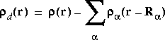
Description
The value refers to the partition function to use in the calculation.![]() a is defined as:
a is defined as:
Eq. 20
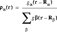 where
where ![]() is an atom index and g
is an atom index and g![]() (r - R
(r - R![]() ) is a function that typically is large for small r - R
) is a function that typically is large for small r - R![]() and small for large r - R
and small for large r - R![]() (i.e., larger near the nucleus). Integrals are rewritten using partition functions as:
(i.e., larger near the nucleus). Integrals are rewritten using partition functions as:
Eq. 21
 which is further reduced to a sum over 3D integration points:
Eq. 22
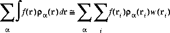 In practice, the partition functions are combined with the integration weights w(ri) to simplify the computation.
Lower_Energy_Limit
Purpose
The Lower_Energy_Limit keyword defines the lower bound of the transition energy range.
Syntax
Lower_Energy_Limit value [units]
Description
If Optical _Absorption is on, the Lower_Energy_Limit and Upper_Energy_Limit keywords control the range of energies within which electronic transitions are computed.
The Rydberg is a fundamental spectroscopic unit (the energy difference between the hydrogen atom 1s ground state level and the continuum is one Rydberg, or half a Hartree).
Max_Loop
Purpose
The Max_Loop keyword specifies the maximum size of the loop size in the numerical integration algorithm.
Syntax
Max_Loop value
| command keyword | values | default | meaning |
|---|---|---|---|
|
Max_Loop
|
integer
|
128
|
Size of loop.
|
Description
You can decrease the amount of memory needed by decreasing the Max_Loop keyword, that is, the maximum size of the loops in the numerical integration algorithm. Smaller loops may be less efficient on vector computers; however, they allow a decrease in the memory required.
Max_Memory
Purpose
The Max_Memory keyword is used to specify the maximum memory (in MBytes) provided for the DMol3 run.
Syntax
Max_Memory value
| command keyword | values | default | meaning |
|---|---|---|---|
|
Max_Memory
|
integer
|
128
|
Size of memory.
|
Description
DMol3 calculates the memory needed, which depends on the size of the system and type of calculation, and compares this with Max_Memory. If the memory needed is greater than Max_Memory, the program stops.
MD_Atom_Mass
Purpose
The MD_Atom_Mass keyword specifies the atomic mass used in the MD run.
Description
Atomic mass can be specified for the MD and Simulated Annealing runs. An example of the use is the study of isotope effects.
MD_Atom_Mass User_Defined 2The first line specifies that mass will be defined for two atoms. The next two lines define atom index 1 and 3 (as they are defined in the .car file) and their masses in AMU.
1 2.0
3 10.0
| command keyword | values | default | meaning |
|---|---|---|---|
|
MD_Time_Step
|
Real value (>0)
|
0.463
|
In femto seconds, this is the time step used in MD. The default time step was set to be 0.463 fs corresponding to the H atom.
|
Description
This is the time step used in the MD propagator. It should be set according to the mass of the lightest atom in the model. Usually, the time step should be proportional to the square root of the atomic mass.
Description
This keyword sets up the initial velocities needed to start the MD or simulated annealing run. The default is using the Maxwell-Boltzmann distribution. To customize the initial velocity, especially for study of chemical reactions, the user can set the specific velocity for each atom. An example of the format in the User_Defined option is as follows:
MD_Velocity User_Defined 3This sets the velocity for three atoms in the molecule, atom index 1, 2 and 5, as it appeared in the .car file. The speed is in Å/ps, the direction of the initial velocity is (1, 0, 0) for atom 1, (-1, 0, 0) for atom 2 and (0, 0, 1) for atom 5. The velocity was computed as the speed x (direction vector), and the direction vector does not need to be unitary.
1 10.0 1.0 0 0
2 10.0 -1.0 0 0
5 5.0 0 0 1.0
Description
The MD_SimAnn_Panel keyword uses a panel of value keywords to control the number of steps, type of propagation and their parameters for each stage of the simulated annealing.
MD_SimAnn_Panel integerThe "integer" specifies n stages in the simulation. The first line is immediately followed by n lines, each defining the parameters for a stage.
index #Step Action Temperature parameter
The "index" is the line number of the list.
The "# Step" is the number of MD steps and is an integer
"Action" may be MD_NVE, MD_NVT, QUENCH, MELT, DAMP, or QUTEMP, as explained in detail below.
"Temperature" is a real number (>0) or the word CONTINUE. CONTINUE begins the panel with the temperature from the last step of the previous panel. You must specify a numeric temperature value for the first panel.
With MD_NVE the constant energy velocity Verlet propagator is used. The generated trajectory samples the micro canonical ensemble.
With MD_NVT, the velocity Verlet propagator was modulated with the Gauss least constraint method to keep the temperature constant. The trajectory generated is isothermic. If you use the MD_NVT parameter, you must also specify the temperature window of variance (typically 1% of the trajectory temperature) by including this parameter after the "Temperature" parameter.
With Quench and Melt, velocity Verlet propagation was used at each time step and the temperature is scaled to vary linearly between the specified temperature (as the initial temperature) and the parameter followed as the final temperature.
With Damp, at each time step, velocity Verlet propagation was used and a finite amount of kinetic energy was withdrawn from the system. Starting with the velocity specified by the temperature, the velocity was then scaled (damped) with the parameter. The parameter should be between 0 and 1, and the closer it is to 0, the steeper the damp. If the value of the parameter is 1, it becomes normal velocity Verlet at constant energy.
With QUTEMP, the velocity Verlet propagation was used at each time step and the temperature is scaled to vary between the specified initial and final temperature following a quadratic function. QUTEMP is not available from the graphical user interface.
|
The molecular dynamics task is equivalent to a single stage simulated annealing task. |
MD_SimAnn_Panel 5The first of the above commands specifies five stages of simulated annealing.
1 200 MD_NVT 300 2.0
2 100 MD_NVE Continue
3 100 Melt 300 1000
4 100 Quench Continue 100
5 100 damp 100 0.2
The second line defines the first stage: 200 time steps of NVT MD at a fixed temperature of 300K. The temperature window is 2K.
The third line defines the second stage: 100 time steps of NVE MD starting with the ending velocity and temperature of the first stage.
The fourth line specifies the third stage: 100 time steps of MD propagation with controlled temperature starting at 300K and rising linearly to reach 1000K at the end.
The fifth line specifies the fourth stage: 100 time steps of MD propagation starting at 1000K and velocity of the last step of the previous panel. The temperature will be decreased linearly to reach 100K at the end of this panel.
The sixth line specifies the fifth stage: 100 time steps of damp propagation starting at 100K. The velocity will be scaled with a factor of 0.2 at each time step.
Description
The coordinates are represented with X, Y and Z.
Example
MD_Fixed_Coordinate 2In the above example there are two atoms with coordinate constraints. Atom 1 has all of the X, Y and Z components fixed, and atom 2 only has the Z component of its Cartesian coordinate fixed.
1 XYZ
2 Z
| command keyword | value keywords | default | meaning |
|---|---|---|---|
|
Memory_Check
|
on
|
|
Calculate memory needed, print a message and stop.
|
|
off
|
|
Don't stop after memory is calculated.
|
Description
If Memory_Check is off, the program continues if the memory needed is less than Max_Memory.
Mulliken_Analysis
Purpose
The Mulliken_Analysis keyword specifies atomic population analysis by the Mulliken method.
Syntax
Mulliken_Analysis value
Description
For a simple Mulliken (1955) analysis (Mulliken_Analysis on), the total effective number of electrons in each atomic orbital is printed. Following this is a reduced or condensed population analysis, giving the total number of electrons in each type of orbital. For example, when using a DN basis, the population analysis gives occupations for two 2s functions, and two 2p functions (for each ml) on every atom. The reduced analysis gives just one 2s, and one 2p population. Following these values comes the effective charge for each atom.
When a population overlap matrix is specified (Mulliken_Analysis population), the orbitals span only the reduced or condensed orbitals; that is, there is only one entry for 1s, 2s, 2p, etc. on each atom, regardless of the size of the atomic basis set.
Nuclear_EFG
Purpose
The Nuclear_EFG keyword specifies calculation of the electric field gradients at nuclei.
Syntax
Nuclear_EFG value
| command keyword | value keywords | default | meaning |
|---|---|---|---|
|
Nuclear_EFG
|
on
|
|
Calculate the EFG.
|
|
off
|
off
|
Do not calculate EFG.
|
Description
When Nuclear_EFG is on, electric field gradients are calculated at the positions of all symmetry-unique nuclei.
Occupation
Purpose
The Occupation keyword specifies orbital occupations and improves SCF convergence.
Syntax
Occupation value_keyword
[ range value_number ...]
Description
DMol3, by default, finds the occupations that yield the lowest energy. This means that electrons occupy orbitals with the lowest orbital energies. The occupation numbers are integers.
Occupation fixed fileThe file filename is rewritten during the SCF cycles with information about the occupation for this particular DMol3 run.
filename
If Fixed is specified, the occupations are entered, in the .occup file in format (15, 2E22.14), as:
N oc odwhere N (an integer) indicates the number of orbitals having this occupation, oc (real number) is the spin-up (alpha) orbital occupation number, and od (real number) is the spin-down (beta) orbital occupation. Terminate the occupation for each irreducible representation with a line containing only a 0. (If you are not using symmetry, there is only one irreducible representation.)
Occupation TOTALIf you are using C2v symmetry, then the occupation of CH2 is 1a12 2a12 3a11 1b12 1b21. The a2 block is unoccupied. The occupation can be specified as:
3 0.10000000000000E+01 0.10000000000000E+01
2 0.10000000000000E+01 0.00000000000000E+00
0
Occupation totalThe order of the representations (a1 a2 b1 b2) is the same as in Cotton (1971) and a list is always printed in the outmol file. Occupations for unused representations should not be specified, and for degenerate representations one should specify occupations only for the first representation.
2 0.10000000000000E+01 0.10000000000000E+01
1 0.10000000000000E+01 0.00000000000000E+00
0
0
1 0.10000000000000E+01 0.10000000000000E+01
0
1 0.10000000000000E+01 0.00000000000000E+00
0
The program writes an .occup file during the SCF cycles. The format of the file is as explained in Examples.
Opt_Constraint
Syntax
Opt_Constraint
constraint specifications ...
blank line
Description and example
The Opt_Constraint keyword is used to specify the distance, angle, and dihedral angle constraints that are to be enforced during a geometry optimization. The constraint specifications are input on separate lines of the input file (immediately following the line containing the Opt_Constraint keyword) and are specified as (in the restricted format (4I4,F20.10)):
atom_i atom_j distanceWhere the atoms are indexed by integers in the order in which they appear in the molecular geometry, distances are expressed in angstroms, and bond angles and dihedral angles are expressed in degrees. The constraint specifications must be terminated with a blank line immediately following the last constraint definition.
atom_i atom_j atom_k angle
atom_i atom_j atom_k atom_l dihedral
<BLANK LINE>
For example, referring to the N-phenylbenzamide geometry (see Basis keyword), the following Opt_Constraint input would define four constraints: the central N2-C1 amide bond distance constrained to 1.336 Å, the C5-N2-C1 angle constrained to 120.0°, the H16-N2-C1-C5 dihedral angle constrained to 168.8°, and the C5-C3 distance constrained to 4.12 Å:
Opt_Constraint
 1  2         1.336
 5  2  1      120.0
 16 2  1  5   168.8
 5  3         4.12
<BLANK LINE>
Description
The Penalty option is more robust, the Lagrange option is more accurate. A constrained transition-state search can be done only with the Lagrange multiplier method--the penalty function algorithm cannot be used.
Opt_Coordinate_System
Purpose
The Opt_Coordinate_System keyword specifies the kind of coordinate system to be used in structure optimization.
Syntax
Opt_Coordinate_System value
Description and example
The Opt_Coordinate_System keyword is used to select the coordinate system in which to carry out the geometry optimization, for example:
Opt_Coordinate_System internal_only
| command keyword | values | default | meaning |
|---|---|---|---|
|
Opt_Displacement_Convergence
|
real
|
0.0011
|
Maximum atomic displacement.
|
| 1
A value smaller than 0.001 is generally too stringent for the DMol default integration grid (medium). You should upgrade the integration mesh (e.g., to fine) if you use values smaller than 0.001.
|
Description and example
The Opt_Displacement_Convergence keyword is used to specify the geometry optimization convergence criterion for the displacement vector, for example:
Opt_Displacement_Convergence 0.0003The displacement criterion is met if the largest (absolute) component of the displacement vector is less than real. The geometry is considered optimized when the gradient convergence criterion (see Opt_Gradient_Convergence keyword) is satisfied and both the displacement convergence and energy convergence criteria (see Opt_Energy_Convergence keyword) are satisfied.
Opt_Energy_Convergence
Purpose
The Opt_Energy_Convergence keyword specifies the threshold for energy convergence during geometry optimization.
Syntax
Opt_Energy_Convergence value
| command keyword | values | default | meaning |
|---|---|---|---|
|
Opt_Energy_Convergence
|
real > 0
|
1.0E-5
|
Energy convergence criterion for geometry optimization.
|
Description
The Opt_Energy_Convergence keyword is used to specify the geometry optimization convergence criterion for the total molecular energy. The energy criterion is met if the difference between the total energy in two consecutive optimization steps is less than real. The geometry is considered optimized when the gradient convergence criterion (Opt_Gradient_Convergence keyword) is satisfied and both the displacement convergence (Opt_Displacement_Convergence) and energy convergence criteria are satisfied.
Opt_Fixed
Syntax
Opt_Fixed
fix coordinate specifications ...
blank line
Description
The Opt_Fixed keyword is used to specify Cartesian constraints (i.e., to constrain the x and/or y and/or z coordinate(s) of specified atom(s)) that are to be enforced during a geometry optimization. The fix coordinate specifications are input on separate lines of the input file (immediately following the line containing the Opt_Fixed keyword) and are specified as (the restricted format (i4,2x,a3) is needed):
Opt_FixedIn this example, atoms 1 and 2 are C and O, respectively, which are allowed to relax during optimization. Atoms 3-7 are fixed Ni atoms.
3 XYZ
4 XYZ
5 XYZ
6 XYZ
7 XYZ
<BLANK LINE>
Description and example
The Opt_GDIIS keyword is used to select the DIIS convergence procedure for geometry optimization, for example:
Opt_GDIIS onNote: GDIIS can be used only for optimizations to minima. Transition-state searches must be done with GDIIS off.
| command keyword | values | default | meaning |
|---|---|---|---|
|
Opt_Gradient_Convergence
|
real > 0
|
1.0E-3
|
Gradient convergence criterion for geometry optimization.
|
Description
The geometry is considered converged to a minimum when the largest (in magnitude) component of the gradient vector is less than Opt_Gradient_Convergence. The geometry is considered optimized when the gradient convergence criterion is satisfied and both the displacement convergence and energy convergence criteria are satisfied (see Opt_Energy_Convergence and Opt_Displacement_Convergence).
Opt_Hessian_Project
Purpose
The Opt_Hessian_Project keyword allows you to specify if any of the 6 frequencies corresponding to translation and rotation of the model are to be removed from the Hessian. For periodic models, the 3 frequencies corresponding to translation can be removed.
Syntax
Opt_Hessian_Project value
| command keyword | value keywords | default | meaning |
|---|---|---|---|
|
Opt_Hessian_Project
|
on or all
|
|
Remove all zero-frequency modes.
|
|
trans
|
|
Remove only translation modes.
| |
|
off
|
|
Do not remove any modes.
|
Description
You should remove all zero-frequency modes during geometry optimizations.
Opt_Hessian_Update
Purpose
The Opt_Hessian_Update keyword controls how the Hessian matrix is updated during the calculation.
Syntax
Opt_Hessian_Update value
Description and example
The Opt_Hessian_Update keyword selects the method for updating the Hessian matrix during a geometry optimization, for example:
Opt_Hessian_Update BFGS
| command keyword | values | default | meaning |
|---|---|---|---|
|
Opt_Iterations
|
integer |
20
|
Controls number of geometry optimization iterations.
|
Description
Geometry optimizations are performed by evaluating a gradient, followed by a Hessian update and calculation of a new set of coordinates. The value of Opt_Iterations controls the number of complete iterations that are performed in a DMol3 run.
Opt_Max_Displacement
Purpose
The Opt_Max_Displacement keyword specifies the maximum allowed step size.
Syntax
Opt_Max_Displacement value
| command keyword | values | default | meaning |
|---|---|---|---|
|
Opt_Max_Displacement
|
real |
0.3
|
Maximum allowed step size.
|
Description and example
The Opt_Max_Displacement keyword is used to specify the maximum length of the geometry update vector, for example:
Opt_Max_Displacement 0.2The value set is the maximum allowed length of the geometry update vector; if the displacement would be larger than real, the step is scaled. For transition-state searches, smaller displacements are recommended (<0.003), especially when no Hessian information is present but the geometry is close to the transition-state geometry.
Description and example
The Opt_Restart keyword is used for reading the starting Hessian matrix for the geometry optimization from a file, for example:
Opt_Restart fileThe file must contain a Hessian matrix in MSI .hessian file format (see file formats documentation at MSI's website at http://www.msi.com/doc/ ). A DMol3 geometry run always produces a new Hessian file that can be used to restart a run.
../archive/ch3nh2.hessian
You can read in a Hessian matrix created with a different program, as long as it is in the correct format. For information on creating a Hessian file from a MOPAC calculation, refer to the section Creating Hessian and Coordinate Files in the MOPAC Interface chapter of this manual.
Opt_Steep_Tol
Purpose
The Opt_Steep_Tol keyword indicates the point at which the geometry optimization algorithm switches to the steepest descents algorithm. If the rms of the gradient is greater than the tolerance, the optimization algorithm uses a steepest descents approach. This is in effect only for geometry optimization.
Syntax
Opt_Steep_Tol value
| command keyword | values | default | meaning |
|---|---|---|---|
|
Opt_Steep_Tol
|
real > 0
|
0.3
|
Switch to steepest descents when gradient rms is greater than real.
|
Description
Steepest descents typically occurs at the beginning of an optimization run, when gradients are large. It can be advantageous then to enable displacement of coordinates solely in the direction of the gradient:
Opt_TS_Mode
Purpose
The Opt_TS_Mode keyword specifies the Hessian mode being followed during a transition-state search.
Syntax
Opt_TS_Mode value
| command keyword | values | default | meaning |
|---|---|---|---|
|
Opt_TS_Mode
|
integer
|
0
|
When Opt_TS_Mode = 0, mode following is switched off and maximization occurs along the lowest mode.
|
Description
You need to start a transition-state search by reading an appropriate Hessian matrix with the Opt_Restart keyword.
Optical _Absorption
Purpose
The Optical_Absorption keyword controls the calculation of optical absorption spectra in DMol3.
Syntax
Optical_Absorption value
| command keyword | value keywords | default | meaning |
|---|---|---|---|
|
Optical_Absorption
|
on
|
|
Calculate optical absorption spectrum.
|
|
off
|
off
|
Do not calculate optical absorption spectrum.
|
Description
If Optical_Absorption is on, the Lower_Energy_Limit and Upper_Energy_Limit keywords control the range of energies within which electronic transitions are computed.
The results are written to the .optabs file. The .optabs file contains two columns: the first for the transition energies, the second for the square of the transition dipole moment associated with the transition energy. Atomic units are used for both the transition energy and the "intensity" (which is reported as the square of the dipole transition moment).
Partial_DOS
Purpose
Setting the Partial_DOS keyword causes the partial density of states coefficients to be written to a run_name.dos file.
Syntax
Partial_DOS value
| command keyword | value keywords | default | meaning |
|---|---|---|---|
|
Partial_DOS
|
on
|
|
Output partial density of states information.
|
|
off
|
off
|
Do not output partial density of states information.
|
Plot
Purpose
The Plot keyword specifies how to compute electronic properties for plotting.
Syntax
Plot value_keyword [# ...] ...
Description
Plot causes DMol3 to generate values of various electronic properties on a 3D grid for subsequent plotting.
Example
To plot the total density, the electrostatic potential, and orbitals 7, 8, and 9, enter:
Plot density potential
Plot orbital 7 8 9
Description
Point charges can be used to simulate the chemical environment due to a large molecule or crystal. The validity of such a calculation depends, of course, on the validity of the point-charge model and the choice of charges used.
Point_Charges filePoint charges can be used in combination with point group symmetry. You need to make sure, however, that the symmetry used in the calculation is a subgroup of the symmetry of both the central molecule and the point charge system.
file_name
Pseudopotential
Purpose
The Pseudopotential keyword specifies the form of core potential or relativistic correction to be used in the calculation.
Syntax
Pseudopotential value
Description
Effective core potentials simplify calculations by combining the effects of many core electrons into a single analytical representation. This can provide a significant speedup without loss of accuracy. At present, ECPs are available for elements Sc through Lr. ECPs also include relativistic effects which are important for heavier elements.
Scalar_Relativity
Purpose
The Scalar_Relativity keyword allows you to use relativistic pseudopotentials. Currently, DMol3 applies scalar relativistic effects, such as Darwin and mass-velocity, in all electron calculations. The properties of these "relativistic" atoms are then reproduced using an essentially nonrelativistic Hamiltonian including pseudopotentials representing scalar relativistic effects.
Syntax
Scalar_Relativity value
| command keyword | value keywords | default | meaning |
|---|---|---|---|
|
Scalar_Relativity
|
off
|
|
No scalar-relativistic effects included.
|
|
on
|
|
Use scalar relativistic effects for all atoms in the model.
|
Description
If Scalar_Relativity is on, then a VPSR file, including pseudopotential information, has to be read from the DMOL3_DATA directory. This option is equivalent to the Pseudopotential VSPR keyword, and is retained for compatibility with DMol 3.5.
Scan_option
Purpose
The Scan_option keyword specifies the type of calculation to be performed at each point of the scan_pes. At this time, only geometry optimizations are supported:
Syntax
SCAN_OPTION optimization
Scan_dim_1
Purpose
The scan_dim_1 keyword specifies the geometric parameters for the first dimension of the Scan_PES calculation. (At this time, only one dimensional scans are supported.)
Syntax
Scan_dim_1
coord_type atom1 atom2 atom3 atom4 start stop steps e
Description
When the value of Calculate is set to Scan_PES, the parameters specified for Scan_dim_1 tell DMol3 how to perform the scan. Use this keyword to specify what type of internal coordinate (Distance, Angle or Dihedral) or which Cartesian coordinate (X, Y, or Z) to scan. The scan will run from the start value to the stop value in steps equal increments. For example, to bend an angle involving atoms numbered 5, 6, and 7 systematically from 80° to 120° in 5 steps, the input would be:
Angle 5 6 7 0 80.0 120.0 5
SCF_Charge_Mixing
Purpose
The SCF_Charge_Mixing keyword specifies the mixing coefficient for the charge density.
Syntax
SCF_Charge_Mixing value1 value2
Description
The mixing coefficient restricts the maximum allowed change in the charge density in the first iterations of the DFT self-consistent procedure, until DIIS becomes active. If ![]() old is the charge density from the previous iteration and
old is the charge density from the previous iteration and ![]() curr is the density in the current iteration, then the new density is:
curr is the density in the current iteration, then the new density is:
Eq. 23
![]() This results in smoother convergence.
This results in smoother convergence.
SCF_CHARGE_MIXING 6 0.000001
| command keyword | values | default | meaning |
|---|---|---|---|
|
SCF_Density_Convergence
|
real > 0
|
1.0E-06
|
SCF density convergence criterion.
|
Description and example
The SCF_Density_Convergence keyword is used to specify the electron density convergence threshold for the SCF procedure, for example:
SCF_Density_Convergence 0.000001The SCF electron density is considered converged when the difference between the norms of the electron density in two successive SCF iterations is less than the value of SCF_Density_Convergence. The density convergence criterion must be satisfied for SCF convergence to be achieved.
In most calculations, an SCF_Density_Convergence value of 10-5 is adequate.
Description and example
This option can significantly improve SCF convergence. For metallic systems it may be necessary to use the SCF_DIIS keyword together with small values of the SCF_Charge_Mixing and SCF_Spin_Mixing parameters. It is not recommended that you use an SCF_DIIS value less than 4.
Normally, an SCF begins with simple mixing. Once the magnitude of the SCF convergence falls below the value specified by the SCF_Charge_Mixing keyword, DIIS is used.
Two different DIIS procedures are available. The pulay option uses the conventional DIIS technique and works well for molecular systems. The kresse technique appears to be a netter option for periodic systems. In the case of the kresse technique, SCF mixing and DIIS extrapolation can be used simultaneously.
SCF_Direct
Purpose
The SCF_Direct keyword is used to specify the direct SCF procedure.
Syntax
Direct value
| command keyword | values | default | meaning |
|---|---|---|---|
|
SCF_Direct
|
on
|
on
|
Use the direct scheme.
|
|
off
|
|
Use the conventional scheme.
|
Description
The numeric integration requires evaluating quantities of the form:
Eq. 24
 This is usually accomplished by storing the value of each atomic orbital
 ![]() µ at each of the DMol integration grid points ri. This information is stored in the file .fwv and is read during each iteration of the SCF procedure. A medium-sized molecule may have about 300 atomic orbitals and 50000 grid points and would require 120 megabytes of disk space.
µ at each of the DMol integration grid points ri. This information is stored in the file .fwv and is read during each iteration of the SCF procedure. A medium-sized molecule may have about 300 atomic orbitals and 50000 grid points and would require 120 megabytes of disk space.
SCF_Iterations
Purpose
The SCF_Iterations keyword is the maximum number of iterations.
Syntax
SCF_Iterations value
| command keyword | values | default | meaning |
|---|---|---|---|
|
SCF_Iterations
|
integer |
25
|
Specify maximum number of iterations allowed in self-consistent solution of DFT equations.
|
Description
Setting SCF_Iterations to larger values results in fuller convergence but added expense. The program exits when the number of iterations is exceeded or when the convergence criterion specified by SCF_Density_Convergence is met, whichever comes first.
A value of SCF_Iterations < 0 means that, regardless of the success of SCF convergence, the program continues after the maximum number of SCF cycles has occurred.
SCF_Number_Bad_Steps
Purpose
The SCF_Number_Bad_Steps keyword specifies the number of allowed bad (divergent) iterations before aborting a run.
Syntax
SCF_Number_Bad_Steps value
| command keyword | values | default | meaning |
|---|---|---|---|
|
SCF_Number_Bad_Steps
|
integer > 0
|
13
|
Limit number of divergent iterations.
|
Description
During the self-consistent procedure, if the mixing factor is too large, the iterations might not converge. SCF_Number_Bad_Steps indicates how many bad steps in a row are permitted before the program aborts the self-consistent procedure. Values of 0 or 1 are not recommended, since the program often takes a single divergent step but recovers on the next iteration.
SCF_Restart
Purpose
The SCF_Restart keyword is used to restart an interrupted or unconverged calculation.
Syntax
SCF_Restart value
Description
Because the .tpotl file contains the analytic representation of the Coulombic potential, restarting from it allows the SCF iterations to pick up where they left off. Alternatively, using an old .tpotl file at a different geometry may give the calculation a better starting guess than the default, the density from the superposition of atomic densities. If the integration grid, symmetry, or basis set is changed, the .tpotl file will no longer be compatible.
SCF_Spin_Mixing
Purpose
The SCF_Spin_Mixing keyword specifies the mixing coefficient for the spin density.
Syntax
SCF_Spin_Mixing value
| command keyword | values | default | meaning |
|---|---|---|---|
|
SCF_Spin_Mixing
|
real |
0.25
|
Restricts maximum allowed change in spin density at the first iteration.
|
Description
The mixing coefficient restricts the maximum allowed change in the spin density at the first iteration of the DFT self-consistent procedure. If ![]() old is the spin density from the previous iteration and
old is the spin density from the previous iteration and ![]() curr is the density in the current iteration, then the new density is:
curr is the density in the current iteration, then the new density is:
Eq. 25
![]() This results in smoother convergence.
This results in smoother convergence.
Spin
Purpose
The Spin keyword specifies twice the z-component of the wave function and is equal to the number of unpaired electrons.
Syntax
Spin value
| command keyword | value keywords | default | meaning |
|---|---|---|---|
|
Spin
|
integer > 0
|
0
|
Value of the spin.
|
Description
If the spin is different than 0, then the calculation results in an excited state with the Spin value being the number of unpaired electrons.
Spin_Polarization
Purpose
The Spin_Polarization keyword controls spin-restricted/unrestricted wavefunctions.
Syntax
Spin_Polarization value
| command keyword | value keywords | default | meaning |
|---|---|---|---|
|
Spin_Polarization
|
restricted
|
restricted
|
Use spin-restricted wavefunctions.
|
|
unrestricted
|
|
Use spin-unrestricted wavefunctions.
|
Description
For spin-restricted wavefunctions, the same orbitals are used for the alpha and beta electrons. For spin-unrestricted wavefunctions, different orbitals are used for different spins.
Start_Spin_Populations
Purpose
The Start_Spin_Populations keyword allows you to input starting spin densities for selected atoms in the model. This option facilitates SCF convergence for ferromagnetic systems and allows for spin localization to occur during bond breaking.
Syntax
Start_Spin_Populations value
[atom_number initial_spin_density
...
blank line]
| command keyword | value keywords | default | meaning |
|---|---|---|---|
|
Start_Spin_Populations
|
off
|
off
|
No initial input spin densities.
|
|
on
|
|
Input the initial spin densities on following lines.
|
Description
When Start_Spin_Populations is on, the input of initial spin densities follows in this format:
Start_Spin_Populations onInput should include all the atoms for which you want to input the initial spin density.
atom_number initial_spin_density
...
<BLANK LINE>
Using the Start_Spin_Population keyword turns on spin-unrestricted calculations.
Start_Spin_Populations onThe 0.5 is used to multiply the atomic spin densities. In this example, at the start of SCF, one of the Cr atoms has positive (up) spin density, and the other has the opposite (down) spin density. This allows for studying the dissociation of the Cr2 model into separate Cr atoms with 6 electrons with spin alpha on one atom and 6 electron of beta spin on the other atom.
1 0.5
2 -0.5
If in this example, Start_Spin_Population were off, DMol3 would try to converge the Cr2 model to an excited state that has the alpha and beta electrons spread equally, so there is no localization of the spin density on any atom.
Note: DMol3 cannot use the Symmetry keyword in conjunction with the Frequency keyword. For Optimize_Frequency or TS_search_frequency calculations, however, DMol3 automatically performs an optimization or transition-state search with the desired symmetry and then a frequency calculation with C1 symmetry.
Description
The coordinates for the model need to be oriented according to certain conventions. This can be done from the Cerius2 interface. When the AUTO (or on) keyword is used, DMol3 detects the symmetry and transforms the coordinates automatically.
The use of symmetry offers several computational advantages. First of all, the secular equation becomes block diagonal. This reduces the size of the matrix diagonalization and subsequently speeds up the calculation. In addition, orbital occupation may be specified for each irreducible representation--this allows the investigation of electronic states of different symmetry. Finally, fewer numerical integration points need to be generated by the program. The points are generated only for a unique region of space, and the full set of points is obtained by symmetry operations. This reduces the computation time and disk storage requirements.
symmetry c2 fixThis allows you to do the calculation with C2 symmetry instead of C2v. DMol3 does not verify if the requested subgroup is indeed a valid choice for the model.
Description
If Optical _Absorption is on, the Lower_Energy_Limit and Upper_Energy_Limit keywords control the range of energies within which electronic transitions are computed.
The Rydberg is a fundamental spectroscopic unit (the energy difference between the hydrogen atom 1s ground state level and the continuum is one Rydberg, or half a Hartree).
Vibration_Project
Purpose
The Vibration_Project keyword specifies to project out translations and rotations from the force-constant matrix.
Syntax
Vibration_Project value
| command keyword | value keywords | default | meaning |
|---|---|---|---|
|
Vibration_Project
|
off
|
|
Do not perform the projection.
|
|
on
|
on
|
Project space of translations and rotations from the force-constant matrix.
|
Description
For molecular models, both translations and rotations are removed; for periodic models, only rotations are removed.
Vibration_Restart
Purpose
The Vibration_Restart keyword restarts a frequency evaluation.
Syntax
Vibration_Restart value
| command keyword | value keywords | default | meaning |
|---|---|---|---|
|
Vibration_Restart
|
on
|
|
Restart a frequency calculation.
|
|
off
|
off
|
Do not restart a frequency calculation.
| |
|
file
|
|
Read .hesswk file.
|
Description
Evaluation of the Hessian by finite differences requires a separate calculation of the gradient for each atom perturbed in each direction x, y, and z. As each gradient is computed, it is stored in the .hesswk file.
Vibration_Restart onthereby not wasting your previous results. DMol3 automatically searches the data in the .hesswk file, identifies the last atom and coordinate for which gradients are available, and restarts the calculation at the next finite displacement. If the .hesswk file contains all the gradients necessary to calculate the second derivatives, DMol3 uses the data in the .hesswk file to compute the vibrational frequencies and evaluate thermodynamic properties.
If the Hessian data are in a file with a name other than run_name.hesswk, say file1, you can ask DMol3 to read that file by specifying:
      Vibration_Restart     file
      file1
Description
Harmonic vibrational frequencies are computed by diagonalizing the mass-weighted second-derivative matrix, F (Wilson et al. 1980). The elements of F are given by:
Eq. 26
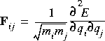 Here, qi and qj represent two Cartesian coordinates of atoms i and j, and mi and mj are the masses of the atoms. The square roots of the eigenvalues of F are the harmonic frequencies.
Eq. 27
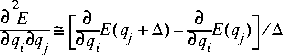 where the two terms represent the analytic derivatives at the equilibrium geometry and at a geometry with coordinate qj displaced by distance
 ![]() .
.
Eq. 28
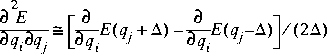 This can reduce numerical rounding-off errors, but takes twice as much computer resources as single-point differencing.