

| Forcefield Based Simulations |
Forcefield-based calculation of relative or absolute free energy should be considered an "expert" application. We recommend using the FDiscover program for relative and absolute free energy calculations. Although it is possible to run relative free energy calculations with CHARMm, that program is slower and less flexible.
To compare chemically distinct systems, the FDiscover program can be used to calculate the relative free energy difference between chemically unique species. This approach uses the finite difference thermodynamic integration (FDTI) algorithm of Mezei et al. (1987). Since FDTI does not require analytical derivatives of the Hamiltonian with respect to the coupling parameter, it is more suited for the complex coupling formalisms required in chemical perturbations. It also has been shown to possess better convergence properties than other methods.
Perturbation method (PM)
The free energy A is related to the partition function Q by the equation:
Eq. 114
![]() If Q1 and Q2 are the partition functions for States 1 and 2, the difference in free energy between these states is:
If Q1 and Q2 are the partition functions for States 1 and 2, the difference in free energy between these states is:
Eq. 115
 Defining Ei(p,r) as the energy function corresponding to state i, the ratio of partition functions is related to the expectation value of exp[-(E2 - E1)/kBT] by:
Eq. 116
 where P1 is the Boltzmann probability function for State 1:
Eq. 117
 This can be expressed more compactly in bracket notation as:
Eq. 118
 where the subscript 1 indicates that State 1 is considered the reference state (that is, the energy difference
  E is computed relative to an ensemble of structures for State 1). Thus, the ratio of the partition functions can be computed from an ensemble average of the energy difference between a reference state and a perturbed state.
Eq. 119
![]() This approach is accurate only when the energy of the initial and final states differs by a small amount, on the order of 2 kBT. Larger energy differences than this lead to such small values for the exponential term that the statistical uncertainty overwhelms the observable. For small changes, this method is very attractive because it calculates the complete free energy difference in one calculation.
This approach is accurate only when the energy of the initial and final states differs by a small amount, on the order of 2 kBT. Larger energy differences than this lead to such small values for the exponential term that the statistical uncertainty overwhelms the observable. For small changes, this method is very attractive because it calculates the complete free energy difference in one calculation.
Thermodynamic integration of the relative free energy assumes that the free energy change can be expressed as an integral:

 can be found, which adequately describes a continuous conversion between the two states, the above equation can be integrated numerically. FDTI employs the perturbation formalism to numerically compute the derivatives of the free energy function with respect to the coupling parameter. Using Eq. 119, it is possible to compute the change in free energy (
 Ai) for a perturbation
 away from the ith
  point (
 i ±
i ± 
 ):
):
Eq. 120
![]() Computing
Computing  Ai for many different values of
  spanning the interval from 0 to 1, dividing each
  Ai by
Ai by 
 , and then numerically integrating over the interval, the total free energy change
  A can be estimated. Mathematically, this is summarized as:
Eq. 121
 where k is the number quadrature points in the numerical integration. Notice that
  Ai \xda
 can be computed both for a forward (+
 ) and a backward (-
 ) perturbation. Computing both at the same time takes no more computer time and is a measure of convergence (both should be equal for suitable values of
 ). The Discover program averages the two values for the instantaneous value of
  A \xda
 at
at  i.
i.
The value of 
 i in Eq. 121 for a given i depends on the numerical integration scheme used. For example, a simple trapezoidal rule approach would make each
 i equal. More sophisticated integration methods may allow each
 i to be different. The FDiscover program uses a Gaussian-Legendre quadrature method (Press 1986) that chooses the values needed, given the total number of intervals specified. Hence, you never explicitly specify the
  intervals.

The first step in any free energy calculation is parameterizing the energy function to provide a continuous change between the thermodynamic states that are being compared. The relative free energy function as implemented in the FDiscover program is parameterized at the level of the forcefield parameters themselves. For example, the energy E of a harmonic bond as a function of the bond length b is:
Eq. 122
![]() where K is the force constant and b0 is the reference bond length. In a free energy calculation E(b) may be different for the initial A and final B states (i.e., each state has different force constants and reference bond lengths). The function is reformulated as a function of the coupling parameter:
where K is the force constant and b0 is the reference bond length. In a free energy calculation E(b) may be different for the initial A and final B states (i.e., each state has different force constants and reference bond lengths). The function is reformulated as a function of the coupling parameter:
Eq. 123
 As
As  changes from 0 to 1, the bond description gradually changes from a State A bond to a State B bond.
Relative free energy--methodology
This describes the steps involved in performing an in vacuo calculation to solve the free energy difference between methanol and ethane.
A seminal free energy calculation reported by Jorgensen and Ravimohan (1985) showed that free energy perturbation techniques seem to accurately predict the difference in solvation energy between methanol and ethane. This calculation has since been repeated in several laboratories, using independent programs and forcefields, and has become a de facto benchmark for free energy calculations (Singh et al. 1987; Fleischman and Brooks 1987).
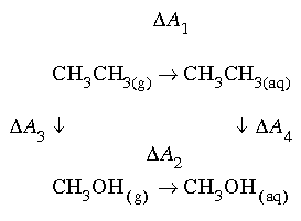
Consider the following thermodynamic cycle for the solvation of ethane and methanol:
|
This cycle requires that:
Eq. 124
![]() The right side of this equation is the difference in solvation free energy that can be measured experimentally. However, the left side is more convenient to compute (making water appear around a solute is a much larger perturbation than changing a methyl group into a hydroxyl group). Either side can be chosen, because both sides are equal.
The right side of this equation is the difference in solvation free energy that can be measured experimentally. However, the left side is more convenient to compute (making water appear around a solute is a much larger perturbation than changing a methyl group into a hydroxyl group). Either side can be chosen, because both sides are equal. A3 is zero and the gas phase calculation can be ignored. Although this is intuitively incorrect, a suitable forcefield could treat the intramolecular energy of ethane and methanol identically. For example, if the nonpolar hydrogens were not represented explicitly, no atom pairs would have more than two intervening bonds. Most forcefields calculate intramolecular nonbond interactions only for atom pairs separated by more than two intervening bonds. Furthermore, if the solutes are treated as rigid models, the energy would not be affected by deformations in bond lengths or angles.
 = 0 and
  = 1 states
To set up the calculation, you must first design the chemical perturbation for methanol going to ethane. You must first choose which of these models corresponds to the
 = 0 state. The
  = 0 state must always have enough atoms to accommodate both molecular extremes, even if invisible "dummy" atoms must be added as placeholders for atoms that appear as the perturbation proceeds.
 = 0 state, because methanol can be completely subsumed within ethane. However, to illustrate that the choice is arbitrary, the calculation in the opposite direction, for methanol going to ethane, is described.
  = 0 state is provided to FDiscover as would any model for simulation, in ordinary coordinate (.car) and molecular data (.mdf) files. In the FDiscover command input file (.inp), you can specify which atoms are being perturbed and their limiting states with the Warp command. The limiting states are defined completely by the potential atom type, the partial atomic charge, and the mass of each atom.
The free energy summary table printed out at the end of the completed free energy loop (after the last resume) contains the complete history. Throughout the run, a partial summary table is output after each resume and contains all the available data.
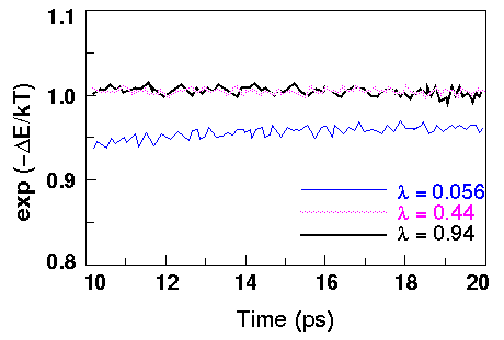
Graphing the Boltzmann factor [exp -(
 E \xda kT)] vs. time aids in assessing convergence during a given calculation. Systematic drift in exp -(
 E \xda kT) over time is symptomatic of nonconvergence.
|
 E \xda kT)] for the first, third, and last
  points for the methanol-to-ethane gas phase calculation. Note that there is a slight upward drift in the curve for the first
  point, although the others seem to have converged.
This section includes
![]()
Absolute free energy
This approach is a special case of the thermodynamic integration approach to free energy calculations, which is itself a general method for computing the change in free energy upon going from one thermodynamic state to another. Absolute free energy simply constrains one of these states to be a model system for which the absolute free energy is known analytically. By integrating from a known, albeit model, state to the final real state, the absolute free energy becomes the sum of the numerically computed thermodynamic integration step and the analytical absolute free energy of the model state.
Uses of absolute free energy calculations
Derivation for ideal systems
The absolute free energy algorithm depends on defining a model for which the partition function in Eq. 114 can be derived analytically. The model implemented in the FDiscover program is an ideal solid. That is, the atoms in the system are constrained harmonically to a lattice (analogous to a solid) and do not interact with each other (analogous to the familiar ideal gas). The Hamiltonian for such a system is:
Eq. 125
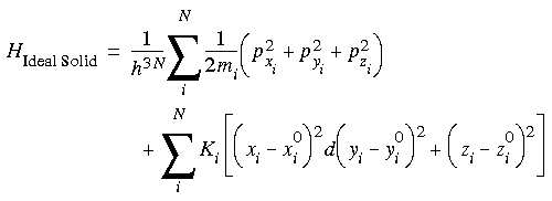 where the first summation is simply the kinetic energy (including a reciprocal of Planck's constant for each degree of freedom, a quantum effect), and the second is a harmonic function constraining each atom to a corresponding lattice point (xi0, yi0, zi0) with a force constant of Ki. Note that there are no terms for interactions between particles. This simplification is what makes an analytical solution possible. Substituting this Hamiltonian into the partition function gives:
Eq. 126
 Returning to Eq. 114, the free energy of the model ideal solid can be written as:
Eq. 127
 A remarkable result of this formula is that it does not depend on coordinates--neither the model coordinates nor the lattice site coordinates. It depends only on the mass of the atoms and the force constant used for the harmonic constraint. This property has important practical implications for free energy calculations, making it possible to choose whatever set of lattice site coordinates gives the best convergence properties for the subsequent thermodynamic integration step.
As shown above, integrating the partition function analytically may be possible for simple Hamiltonians. However, for more realistic systems that include many nonbond and bond interactions between atoms, an analytic solution is impossible. As in the relative free energy calculation (see FDTI), we use thermodynamic integration to determine the change in free energy:
Eq. 128
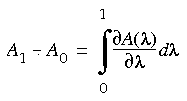 Substituting the equation for the free energy (Eq. 114) into Eq. 128, we can write the difference in free energy as a function of the partition function Q(
 ):
):
Eq. 129
 Without defining explicitly how the Hamiltonian depends on
  , we can write the difference in the energies as:
Eq. 130
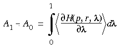 The problem of computing a free energy difference is thus simplified to that of computing the expectation value of a derivative of the Hamiltonian. Since an expectation value is, according to Gibbs' postulate (an axiom of statistical mechanics), the ensemble average of the quantity, it is easily computed as the average of that quantity over a suitably equilibrated set of snapshots of the system.
Eq. 130 is perfectly general for any classical system and is the fundamental equation of all thermodynamic integration methods. However, we have not yet described what the Hamiltonian is or how it can be parameterized in terms of  . The Hamiltonian could be parameterized in an infinite number of ways. Because a function of state (the free energy) is being integrated, the path between the end points is arbitrary. For absolute free energy calculations, it turns out that the simplest form is perfectly adequate.
The parameterization scheme adopted by the FDiscover program is straightforward. The Hamiltonian is defined as a linear combination of the two potential energy functions that describe the extreme states:
Eq. 131
![]() Here, K(p) is the kinetic energy (because the two states are completely defined by their respective potential energy functions, the kinetic energy does not have to be coupled to
Here, K(p) is the kinetic energy (because the two states are completely defined by their respective potential energy functions, the kinetic energy does not have to be coupled to  ), V0 is the normal potential energy function (including bonds, angles, torsions, etc.), and VH is a harmonic oscillator site potential given by:
Eq. 132
 Parameterization of the Hamiltonian
where Ki is the ith atom's spring constant, ri is the ith atom's instantaneous coordinate, and ri0 the reference lattice of the noninteracting atoms (often referred to as an Einstein solid). This choice of parameterization is motivated by the template-forcing concept in the FDiscover program and by previous free energy evaluations (Hoover and Ree 1967). In Eq. 131,  is greater than 0 and less than 1, and describes an energy-space path between a system described by an unadulterated molecular forcefield (
 = 0) and one represented by independent harmonic oscillators (
 = 1).
= 1).
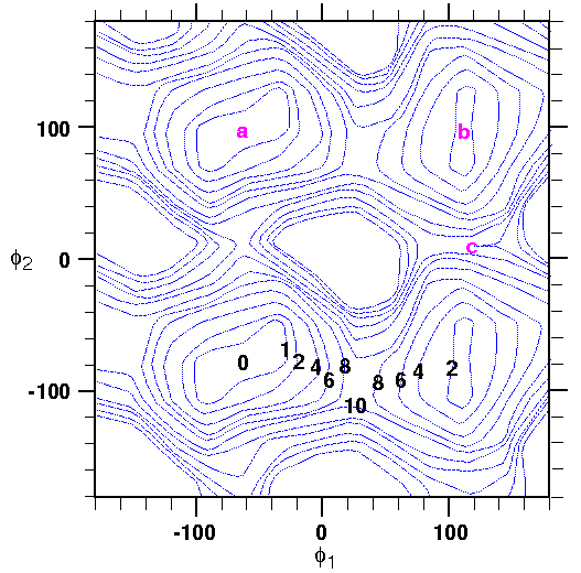
Eq. 132 is thus the reference system for which an absolute free energy can be directly calculated. The potential VH restricts the exploration of phase space to a region defined by atomic mean-squared displacements relative to the Einstein solid. Consequently, the choice of both the reference state and spring constants, in general, affects the calculated free energies. For most cases, the energy-minimized coordinates of a mechanically stable structure are used for the reference Einstein solid. Using Eq. 127 for the free energy of the Einstein solid A1 and Eqs. 130 through 132, the absolute free energy of the real state is:
Absolute free energy of the real state
Eq. 133
 Computational considerations and precautions
The simple form of Eq. 133 makes evaluating its ensemble average straightforward. A comprehensive dynamics trajectory for a given value of  represents an ensemble of structures for that
  . By computing and averaging the values of (V0 - VH) for each structure in this ensemble, the integrand can be numerically estimated for any given value of
  . By performing several such calculations for many values of
  between 0 and 1, eventually the function can be numerically integrated.
Several practical simulation considerations are apparent from Eqs. 131 and 133.
For example, when  is close to zero, the calculated ensemble of structures includes configurations far from the reference state (the ensemble is generated according to Eq. 131). Therefore, fluctuations of VH are large when VH is evaluated for this ensemble.
Conversely, when  is close to one, the structures generated are minimally influenced by the real forcefield. These ensembles can include structures with distorted bonds, angles, and even overlapping atoms, leading to large fluctuations in V0 in Eq. 133. Large fluctuations of (V0 - VH) decrease the precision with which its integral can be calculated. The overall effect is to destabilize the integral and, in extreme cases, cause it to diverge.
These undesirable effects can be minimized by reasonable choices of reference structures, spring constants, and integration algorithm. For example, the FDiscover program uses a Gaussian-Legendre quadrature algorithm to integrate Eq. 133. This has the useful property that one need not evaluate the function at the boundaries (where the divergence is worst).
The choice of the reference state is the most critical step in an absolute free energy calculation. The reference state determines where the sampling of configuration space is centered. Choosing reference states that are only slightly different (for example, 0.1 Å rms in coordinates) can change the free energy significantly if the reference state has any residual strain.
The absolute free energy technique is primarily used to evaluate the free energy of different conformations of the same model. This is particularly difficult to do by perturbation methods alone, since a path from one conformation to another may be difficult to construct and model (for example, a path converting an
 -helix into a
  -sheet). Although free energy methods are path independent (because what is being evaluated is the difference between thermodynamic state functions), the integration through the path must be performed reversibly, which is problematic for large structural rearrangements.
Example: Fentanyl
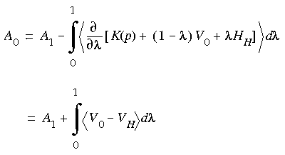
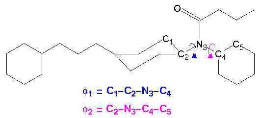
This example presents a calculation of the free energies of various conformational states of fentanyl (Figure 33
|
|
The reference state has two roles in the free energy calculation. A trivial contribution is the free energy it contributes as an ideal solid. This contribution is trivial because it does not depend on the conformation of the reference structure. It depends only on the masses of its atoms and the spring constants constraining each atom to the lattice (see Eq. 127).
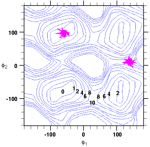
The nontrivial role is that it determines which part of configurational space is sampled during dynamics. In this example, the free energies of states a, b, and c (Figure 34) of fentanyl are compared. The reference states for a and b correspond to completely minimized structures at these points. Point c in Figure 34 represents the free energy at a barrier. Obviously, it would be incorrect to minimize this reference structure--it would simply roll down into one of the adjacent wells. The lowest-energy structure at the saddle point can be constructed by forcing the dihedral angles to adopt the values of the saddle point (using the force torsion command in the standalone version of the FDiscover program, or the Constraint/TorsionForce command in the Insight version) while minimizing the rest of the model (this, of course, is how the energy map in Figure 34 was generated in the first place).
It is important to choose the lowest-energy structure consistent with a given conformational state, so that the free energy calculated does not contain excess enthalpy. Constraining the sampling of configurational space to a rather small region localized around the reference structure limits the distribution of energies that is sampled. Moving the reference structure to a slightly higher-energy conformation would sample different energies and change the total free energy.
 1 and
1 and  2 is superimposed on the
  1 \xda
  2 energy map for one of the
  ensembles. Note how only the local region around the reference structure is sampled. While this may be unsettling (what is the meaning of a free energy that does not represent all of configurational space), remember that you are interested in the difference in free energy between closely related states (a, b, and c differ mainly by rotation of two dihedral angles). To achieve this resolution, the sampling must be restricted accordingly.
|
Hints for setting up the absolute free energy calculation
In the Insight version of the FDiscover program, an absolute free energy calculation is set up using the Parameters/Absolute command. The system is first minimized, then the atoms are tethered to the minimized locations. The Parameters/Minimize and Parameters/Dynamics commands can be used to control the initial minimization, as well as the dynamics used to sample the conformational space.
The spring constants also affect the error associated with a calculation. Ensembles that contain structures far from the reference state make greater contributions to the free energy, by virtue of the greater fluctuations in (V0 - VH) for this ensemble.

 -helix or hairpin structures of decaglycine. Typical values of the spring constants range from 1 to 50 kcal mol-1 Å-1.
If possible, you should let Method 2 choose the spring constants automatically. However, if the conformational state is not in a local minimum, you must explicitly specify a spring constant. An estimated value corresponding to a nearby minimum is a good starting point. The error associated with an explicit choice should be monitored, as well as the configurational space sampled for this calculation. Error analysis is discussed under Analysis of results.
Another choice that has to be made is how many
 intervals to use in the integration. This of course depends ultimately on the level of precision needed and the behavior of the integral and cannot be anticipated for all cases.
 ) must be examined. Rapid changes in (V0 - VH) are indicative of systematic errors. Some regions of the integral may need to be computed for longer times and with more intervals, to achieve the desired accuracy.
 intervals typically ranges from 4 to 12. If adequate precision cannot be achieved with 12 intervals, look for and correct systematic factors destabilizing the integral (i.e., Are the spring constants too weak? Is the reference state at too high an energy? Is the system completely equilibrated?).
Analysis of results
Available output
Although a free energy calculation is done as a single FDiscover run, the calculation actually consists of several independent cycles of dynamics equilibration (initialize dynamics) and data collection (resume dynamics)--as many cycles as
 intervals. The results of these dynamics calculations are stored independently for each
  value, in three files.
  cycles. However, the incomplete table is output at the end of each
  interval as an intermediate result.
 ). The frequency of output into this file is controlled by the sampling option in the absolute free energy command and is, by default, output every step. The .tot file is particularly convenient as input to plotting and statistical analysis programs (such as SAS or RS1).
  run. Because a free energy calculation consists of several
  cycles, each with its own initialize command, there can be several history files. To allow for several history files with the same root name, an option has been added to the initialize command to change the extension from .his to a number (e.g., FENTANYL.1, FENTANYL.2, etc.). This is specified by including the keyword save in the initialize command. If save is not included, the Discover program keeps only the history file corresponding to the last
  run.
run.
A major source of systematic error in these calculations is lack of convergence (that is, failure to equilibrate long enough to achieve thermodynamic equilibrium at each
 value) and insufficient sampling of configurational space. Other sources of systematic error include inaccuracies in the force field (both in the functional form and the parameters) and quantum mechanical effects.
  value.
Careful analysis of the random errors reported by the FDiscover program helps point to likely systematic errors. For example, rapid changes in error as a function of
 could be caused by a failure to completely equilibrate.
  = 0.8. It is wasteful to compute all intervals at the worst-case level.
 = 0 to 0.8. The second calculation would compute the free energy from
  = 0.8 to 1.0 with longer equilibration and sampling times.
Eq. 135
 Absolute free energy files and output
The .cli file contains the free energy comparison list, i.e., the template coordinates prevalent during tethering. This file can be used as input for further simulations with the same template coordinates, by specifying file filename with the calculate command in the standalone version of the FDiscover program.
A table of spring constants is printed before commencing the first dynamics simulation for the integration over
 . The data tabulated are absolute atom #, harmonic force constant, and (optionally) mean-square displacement and mean harmonic energies as deduced from spring-constant-generation procedures utilizing molecular dynamics.
Dynamics running averages contain additional categories for (V0 - VH) and <V0>.

Each table of dynamics averages generated by resume is followed by a table summarizing contributions to the free energy integral, including statistical errors and variances on the value dF for each lambda value.
 = 1 state of the template). Each
  value has an associated output table in the .out file.
