
| Forcefield Based Simulations |
Who should read this chapter
You should read this chapter if you want to know:
Related information
Preparing the Energy Expression and the Model presents information on how the functional forms of forcefields are used for real simulations. You need to read it to optimize how you set up your simulation. The general procedure for forcefield-based calculations is outlined under Using forcefields.
The atom types defined for each forcefield are listed under Forcefield Terms and Atom Types. Illustrations of various types of cross terms are also included.
The files that specify the forcefields are described in the separate documentation for each simulation engine.
The complete mathematical description of a molecule, including both quantum mechanical and relativistic effects, is a formidable problem, due to the small scales and large velocities. However, for this discussion, these intricacies are ignored and the focus is on general concepts, because molecular mechanics and dynamics are based on empirical data that implicitly incorporate all the relativistic and quantum effects. Since no complete relativistic quantum mechanical theory is suitable for the description of molecules, this discussion starts with the nonrelativistic, time-independent form of the Schrödinger description:![]()
The potential energy surface
Eq. 1
![]() where H is the Hamiltonian for the system,
where H is the Hamiltonian for the system,  is the wavefunction, and E is the energy. In general, is a function of the coordinates of the nuclei (R) and of the electrons (r).
Although this equation is quite general, it is too complex for any practical use, so approximations are made. Noting that the electrons are several thousands of times lighter than the nuclei and therefore move much faster, Born and Oppenheimer (1927) proposed what is known as the Born-Oppenheimer approximation: the motion of the electrons can be decoupled from that of the nuclei, giving two separate equations. The first equation describes the electronic motion:
Eq. 2
![]() and depends only parametrically on the positions of the nuclei. Note that this equation defines an energy E(R), which is a function of only the coordinates of the nuclei. This energy is usually called the potential energy surface.
and depends only parametrically on the positions of the nuclei. Note that this equation defines an energy E(R), which is a function of only the coordinates of the nuclei. This energy is usually called the potential energy surface.
The second equation then describes the motion of the nuclei on this potential energy surface E(R):
Eq. 3
![]() The direct solution of Eq. 2 is the province of ab initio quantum chemical codes such as Gaussian, CADPAC, Hondo, GAMESS, DMol, and Turbomole. Semiempirical codes such as ZINDO, MNDO, MINDO, MOPAC, and AMPAC also solve Eq. 2, but they approximate many of the integrals needed with empirically fit functions. The common feature of these programs, though, is that they solve for the electronic wavefunction and energy as a function of nuclear coordinates. In contrast, simulation engines provide an empirical fit to the potential energy surface.
The direct solution of Eq. 2 is the province of ab initio quantum chemical codes such as Gaussian, CADPAC, Hondo, GAMESS, DMol, and Turbomole. Semiempirical codes such as ZINDO, MNDO, MINDO, MOPAC, and AMPAC also solve Eq. 2, but they approximate many of the integrals needed with empirically fit functions. The common feature of these programs, though, is that they solve for the electronic wavefunction and energy as a function of nuclear coordinates. In contrast, simulation engines provide an empirical fit to the potential energy surface.
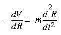
Solving Eq. 3 is important if you are interested in the structure or time evolution of a model. As written, Eq. 3 is the Schrödinger equation for the motion of the nuclei on the potential energy surface. In principle, Eq. 2 could be solved for the potential energy E, and then Eq. 3 could be solved. However, the effort required to solve Eq. 2 is extremely large, so usually an empirical fit to the potential energy surface, commonly called a forcefield (V), is used. Since the nuclei are relatively heavy objects, quantum mechanical effects are often insignificant, in which case Eq. 3 can be replaced by Newton's equation of motion:![]()
Empirical fit to the potential energy surface
Eq. 4
 Molecular dynamics and mechanics
The solution of Eq. 4 using an empirical fit to the potential energy surface E(R) is called molecular dynamics. Molecular mechanics ignores the time evolution of the system and instead focuses on finding particular geometries and their associated energies or other static properties. This includes finding equilibrium structures, transition states, relative energies, and harmonic vibrational frequencies.
The forcefield
Components of a forcefield
The forcefield contains the necessary building blocks for the calculations of energy and force:
Coordinates, terms, functional forms
The forcefields commonly used for describing molecules employ a combination of internal coordinates and terms (bond distances, bond angles, torsions, etc.), to describe part of the potential energy surface due to interactions between bonded atoms, and nonbond terms to describe the van der Waals and electrostatic (etc.) interactions between atoms. The functional forms range from simple quadratic forms to Morse functions, Fourier expansions, Lennard-Jones potentials, etc.
The goal of a forcefield is to describe entire classes of molecules with reasonable accuracy. In a sense, the forcefield interpolates and extrapolates from the empirical data of the small set of models used to parameterize the forcefield to a larger set of related models. Some forcefields aim for high accuracy for a limited set of element types, thus enabling good prediction of many molecular properties. Other forcefields aim for the broadest possible coverage of the periodic table, with necessarily lower accuracy.
The physical significance of most of the types of interactions in a forcefield is easily understood, since describing a model's internal degrees of freedom in terms of bonds, angles, and torsions seems natural. The analogy of vibrating balls connected by springs to describe molecular motion is equally familiar. However, it must be remembered that such models have limitations. Consider for example the difference between such a mechanical model and a quantum mechanical "bond".
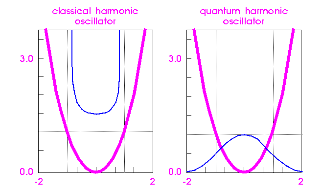
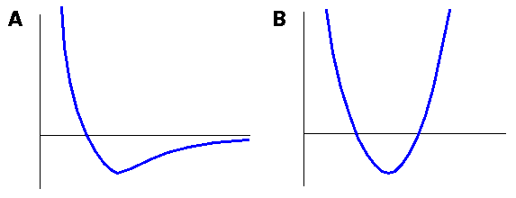
Covalent bonds can, to a first approximation, be described by a harmonic oscillator, both in quantum and classical mechanical theory. Consider the classic oscillator in Figure 1. A ball poised at the intersection of the pale horizontal line with the parabolic energy surface (thick line) would begin to roll down, converting its potential energy to kinetic energy and achieving a maximum velocity as it passes the minimum. Its velocity (kinetic energy) is then converted back into potential energy until, at the exact same height as it had started, it would pause momentarily before rolling back. The interchange of kinetic and potential energy in such a mechanical system is familiar and intuitive.
The probability of finding the ball at any point along its trajectory is inversely proportional to its velocity at that point (which is opposite to the probability for a real atom). This probability is plotted above the parabolic curve (thin line, Figure 1). The probability is greatest near the high-energy limits of its trajectory (where it is moving slowly) and lowest at the energy minimum (where it is moving quickly). Because the total energy cannot exceed the initial potential energy defined by the starting point, the probability drops to zero outside the limit defined by the intersection of the total energy (pale horizontal line) with the parabola.
The energy is indicated by the heavy lines and probability by the thin lines. The total energy of the system is indicated by the pale horizontal line. The classical (mechanical) probability is highest when the particle reaches it maximum potential energy (zero velocity) and drops to zero between these points. The quantum mechanical probability is highest where the potential energy is lowest, and there is a finite probability that the particle can be found outside the classical limits (pale vertical lines).
Figure 1. Energy and probability of a mechanical and quantum particle in a harmonic energy well
|
Describing a quantum mechanical "trajectory" is impossible, because the uncertainty principle prevents an exact, simultaneous specification of both position and momentum. However, the probability that the quantum mechanical ball will be at a given point on the parabola can be quantified. The quantum mechanical probability function plotted in the right panel of Figure 1 is very different from the mechanical system. First, the highest probability is at the energy minimum, which is the opposite of the mechanical case. Second, the quantum mechanical ball can actually be found beyond the classical limits imposed by the total energy of the system (tunneling). Both these properties can be attributed to the uncertainty principle.
Utility of the forcefield approach
With such a different qualitative picture of fundamental physical principles, is it reasonable to use a mechanical approach for obviously quantum mechanical entities like bonds? In practice, many experimental properties such as vibrational frequencies, sublimation energies, and crystal structures can be reproduced with a forcefield, not because the systems behave mechanically, but because the forcefield is fit to reproduce relevant observables and therefore includes most of the quantum effects empirically. Nevertheless, it is important to appreciate the fundamental limitations of a mechanical approach.
Applications beyond the capability of most forcefield methods include:
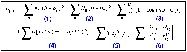
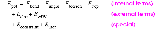
The potential energy of a system can be expressed as a sum of valence (or bond), crossterm, and nonbond interactions:
Valence interactions
The energy of valence interactions is generally accounted for by diagonal terms, namely, bond stretching (Ebond), valence angle bending (Eangle), dihedral angle torsion (Etorsion), and inversion (also called out-of-plane interactions) (Einversion or Eoop) terms, which are part of nearly all forcefields for covalent systems. A Urey-Bradley term (EUB) may be used to account for interactions between atom pairs involved in 1-3 configurations (i.e., atoms bound to a common atom):
Eq. 5
Evalence = Ebond + Eangle + Etorsion + Eoop + EUB
Valence crossterms
Modern (second-generation) forcefields generally achieve higher accuracy by including cross terms to account for such factors as bond or angle distortions caused by nearby atoms. Crossterms can include the following terms: stretch-stretch, stretch-bend-stretch, bend-bend, torsion-stretch, torsion-bend-bend, bend-torsion-bend, stretch-torsion-stretch. (These are illustrated under Forcefield Terms and Atom Types.)
The energy of interactions between nonbonded atoms is accounted for by van der Waals (EvdW), electrostatic (ECoulomb), and (in some older forcefields) hydrogen bond (Ehbond) terms:
Eq. 6
Enonbond = EvdW + ECoulomb + Ehbond
Restraints
Restraints that can be added to an energy expression include distance, angle, torsion, and inversion restraints. Restraints are useful if you, for example, are interested in the structure of only part of a model. For information on restraints and their implementation and use, see Preparing the Energy Expression and the Model in this documentation set and also the documentation for the particular simulation engine.
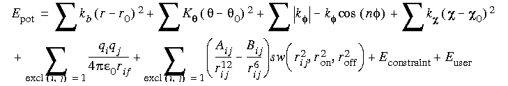
Example energy expression for water
As a simple example of a complete energy expression, consider the following equation, which might be used to describe the potential energy surface of a water model:
Eq. 7
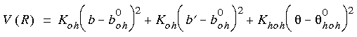 where Koh, b0oh, Khoh, and
  0hoh are parameters of the forcefield, b is the current bond length of one O-H bond, b´ is the length of the other O-H bond, and is the H-O-H angle.
0hoh).
Eq. 7 is an example of an energy expression as set up for a simple molecule. Eq. 8 is an example of the corresponding general, summed forcefield function:
Eq. 8
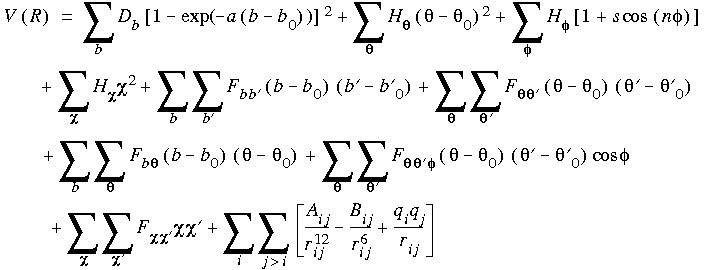
The first four terms in this equation are sums that reflect the energy needed to stretch bonds (b), bend angles () away from their reference values, rotate torsion angles ( ) by twisting atoms about the bond axis that determines the torsion angle, and distort planar atoms out of the plane formed by the atoms they are bonded to (
 ). The next five terms are cross terms that account for interactions between the four types of internal coordinates. The final term represents the nonbond interactions as a sum of repulsive and attractive Lennard-Jones terms as well as Coulombic terms, all of which are a function of the distance rij between atom pairs. The forcefield defines the functional form of each term in this equation as well as the parameters such as Db,
  , and b0. The forcefield also defines internal coordinates such as b, , , and as a function of the Cartesian atomic coordinates, although this is not explicit in Eq. 8.
We should note that the energy expression in Eq. 8 is cast in a general form. The true energy expression for a specific model includes information about the coordinates that are included in each sum. For example, it is common to exclude interactions between bonded and 1-3 atoms in the summation representing the nonbond interactions. Thus, a true energy expression might actually use a list of allowed interactions rather than the full summation implied in Eq. 8.
The results of any mechanics or dynamics calculation depend crucially on the forcefield. The quality of the description of both the system and the particular properties being analyzed is of paramount importance. Accurate, specific parameters generally give better results than automatic, generic parameters. Choosing the correct forcefield is vitally important in getting reasonable results from energy calculations.![]()
Forcefields supported by MSI forcefield engines
This section gives a general comparison of the forcefields that are available in MSI products and presents the reasoning behind making a wide variety of forcefields available to our customers. It should enable you to make at least a preliminary choice of which forcefield to use.
Complete descriptions of each forcefield follow in subsequent sections:
The atom types defined by each forcefield are listed under Forcefield Terms and Atom Types, and the types of parameters used in the forcefields are described in the documentation for each simulation engine.
Main types of forcefields
MSI provides four main types of forcefields:
In addition, we supply (but do not support) several older or untested forcefields.
Additional information about forcefields included with Cerius2 is printed to the text window when you load a forcefield. Alternatively, you can click the Show information action button in the Load Force Field control panel.
Availability
![]()
Second-generation forcefields accurate for many properties
The topography of an energy surface is usually very complex, especially for large and/or complex models, with many energy minima and barriers and regions of greatly varying energy and curvature. Nevertheless, the forcefield expression must be as accurate and complete as possible, to avoid spurious or misleading results. The newer, second-generation forcefields meet this requirement through their greater complexity than the classical forcefields, having expanded analytic energy expressions that include additional terms.
The complexity of second-generation forcefields requires the use of a large number of forcefield parameters. There are almost always far more parameters than can be inferred from experiment, such as by microwave or infrared spectroscopy. However, modern quantum mechanical methods can generate enough quantum observables so that all the necessary parameters can be accurately determined by fitting the energy expression to these observables.
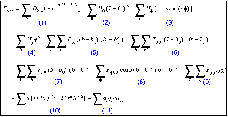
Advantages of deriving forcefields from quantum calculations
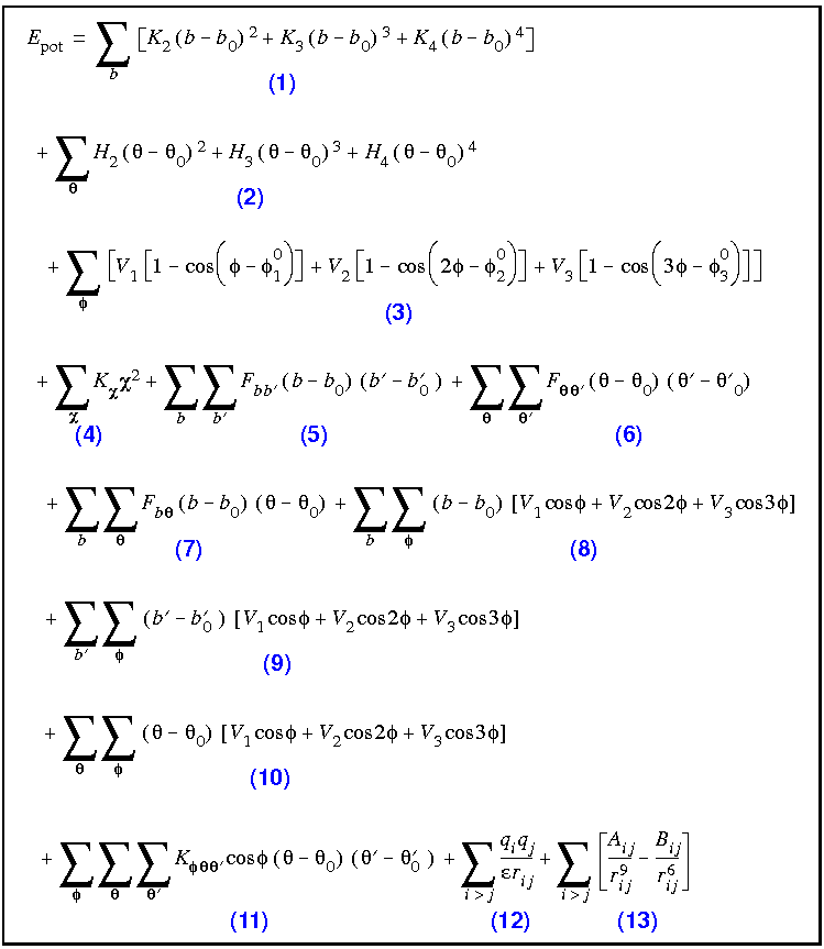
The analytic expressions used to represent the energy surface are shown in Eq. 9. Both anharmonic diagonal terms and many crossterms are necessary for a good fit to a variety of structures and relative energies, as well as to vibrational frequencies.
The CFF forcefields employ quartic polynomials for bond stretching (Term 1) and angle bending (Term 2) and a three-term Fourier expansion for torsions (Term 3). The out-of-plane (also called inversion) coordinate (Term 4) is defined according to Wilson et al. (1980). All the crossterms up through third order that have been found to be important (Terms 5-11) are also included--this gives a forcefield equivalent to the best used in a formate anion test case (Maple et al. 1990). Term 12 is the Coulombic interaction between the atomic charges, and Term 13 represents the van der Waals interactions, using an inverse 9th-power term for the repulsive part rather than the more customary 12th-power term.
Note
|
Because the Wilson out-of-plane definition is used in the CFF family of forcefields, results calculated with CDiscover, FDiscover, and Cerius2·OFF should agree exactly. |
Eq. 9
CFF91 forcefield
Applicability
CFF91 is useful for hydrocarbons, proteins, protein-ligand interactions. For small models it can be used to predict: gas-phase geometries, vibrational frequencies, conformational energies, torsion barriers, crystal structures; for liquids: cohesive energy densities; for crystals: lattice parameters, rms atomic coordinates, sublimation energies; for macromolecules: protein crystal structures.
The functional form of CFF91 is exactly as shown in Eq. 9.
CFF91 has parameters for functional groups that consist of H, Na, Ca, C, Si, N, P, O, S, F, Cl, Br, I, and/or Ar. The atom types of the CFF91 forcefield are listed in Table 27.
The bond increment section of the .frc file for CFF91 enables partial charges to be determined whenever the Discover program or the Cerius2·OFF module is able to assign automatic atom types.
CFF forcefield
Applicability
CFF (formerly CFF95) was parameterized for additional functional groups beyond CFF91 (Maple et al. 1994a, b, Hwang et al. 1994, Hagler & Ewig 1994). It is recommended for all life sciences applications and for organic polymers such as polycarbonates and polysaccharides.
The atom types of the CFF forcefield are listed in the separate documentation for CFF (below).
Additional information on CFF, which is sold as a separately licensed product, is contained in the MSI Forcefields:CFF book (published separately by MSI).
PCFF forcefield for polymers and other materials
Applicability
PCFF was developed based on CFF91 and is intended for application to polymers and organic materials. It is useful for polycarbonates, melamine resins, polysaccharides, other polymers, organic and inorganic materials, about 20 inorganic metals, as well as for carbohydrates, lipids, and nucleic acids and also cohesive energies, mechanical properties, compressibilities, heat capacities, elastic constants. It handles electron delocalization in aromatic rings by means of a charge library rather than bond increments.
Parameterization, testing, and validation of PCFF included the compounds listed for CFF91 and these functional groups: carbonates, carbamates, phosphazene, urethanes, siloxanes, silanes, ureas (Sun et al. 1994, Sun 1994, 1995), and zeolites (Hill and Sauer 1994). Metal parameters (listed below) were derived by fitting to crystal structures and elastic constants.
PCFF has parameters for functional groups that consist of those listed for CFF91 and also He, Ne, Kr, Xe. In addition, it includes Lennard-Jones parameters for the metals Li, K, Cr, Mo, W, Fe, Ni, Pd, Pt, Cu, Ag, Au, Al, Sn, Pb. Atom type coverage in PCFF includes those listed for CFF91 (Table 27) and the atoms listed here.
COMPASS forcefield for organic and inorganic materials
A high quality general forcefield
COMPASS (Condensed-phase Optimized Molecular Potentials for Atomistic Simulation Studies) represents a technology break-through in forcefield method. It is the first ab initio forcefield that enables accurate and simultaneous prediction of gas-phase properties (structural, conformational, vibrational, etc.) and condensed-phase properties (equation of state, cohesive energies, etc.) for a broad range of molecules and polymers. It is also the first high quality forcefield to consolidate parameters of organic and inorganic materials.
COMPASS is an ab initio forcefield -- most parameters were derived based on ab initio data. Generally speaking, the parameterization procedure can be divided into two phases: ab initio parameterization and empirical optimization. In the first phase, partial charges and valence parameters were derived by fitting to ab initio potential energy surfaces. At this point, the van der Waals parameters were fixed to a set of initial approximated parameters. In the second phase, emphasis is on optimizing the forcefield to yield good agreement with experimental data. A few critical valence parameters were adjusted based on the gas phase experimental data. More importantly, the van der Waals parameters were optimized to fit the condensed-phase properties. For covalent molecular systems, this refinement was done based on molecular dynamics simulations of liquids; for inorganic systems, this is based on energy minimization on crystals.
The parameters for covalent molecules have been thoroughly validated using various calculation methods including extensive MD simulations of liquids, crystals, and polymers. (Sun 1998, Sun et al., 1998, Rigby et al. 1998). For the inorganic materials, validations of COMPASS were performed based on energy minimization method.
The COMPASS forcefield has broad coverage in covalent molecules including most common organics, small inorganic molecules, and polymers. For these molecular systems, the COMPASS forcefield has been parameterized to predict various properties for molecules in isolation and in condensed phases. The properties include molecular structures, vibrational frequencies, conformation energies, dipole moments, liquid structures, crystal structures, equations of state, and cohesive energy densities. The latest development in COMPASS extended the coverage to include inorganic materials - metals, metal oxides, and metal halides using various non-covalent models. Currently, some of these materials have been parameterized. COMPASS is able to predict various solid-state properties: unit cell structures, lattice energies, elastic constants, and vibrational frequencies. The combination of parameters for organics and for inorganics opens up the possibility of future study of interfacial and mixed systems.
The COMPASS forcefield is licensed and related files are encrypted. You must have a license for this forcefield in order to use it. The parameters of encrypted forcefields may be viewed with the forcefield editor, but it is not possible to save changes made to the forcefield.
For more information about the COMPASS forcefield, please see the COMPASS user guide.
MMFF94 and MMFF94s, the Merck molecular forcefield
The Merck molecular forcefield is derived largely from ab initio
calculations and can be accurately applied to a variety of condensed-phase
and aqueous systems. It uses a unique functional form for describing the
van der Waals interactions (Halgren 1996a - 1996e, 1999a - 1999b) and employs novel
combination rules that systematically correlate van der Waals parameters
with those that describe experimentally characterized interactions
involving rare-gas atoms. Electrostatic interactions are scaled to mimic
solution effects.
Conformational energies, geometries, and vibrational frequencies of small organic molecules.
The MMFF94 energy expression is similar to that of MM2 and MM3:
Eq. 10
 Where:
 180°).
Charges are implemented via bond increments (similar to CVFF or the CFF family of forcefields) that are included as part of the forcefield.
Missing parameters are supplied via a generic step-down and equivalency typing scheme (see Preparing the Energy Expression and the Model).
The terms of the energy expression are calculated in kcal mol-1. They are described in detail by Halgren (1992, 1996a-d, Halgren & Nachbar, 1996).
Availability
![]()
Rule-based forcefields broadly applicable to the periodic table
Although the second-generation (Second-generation forcefields accurate for many properties) and classical (Classical forcefields) forcefields derive the forcefield parameters by fitting ab initio and/or experimental data sets, these rule-based forcefields rely on atomic parameters coupled with theoretically and empirically derived rules for generating explicit forcefield parameters. The rules embody physical reality (electronegativity, hardness, atomic radii for UFF and ESFF, simple hybridization for Dreiding) and therefore tend to break redundancies and guarantee transferability. As much as possible, the atomic parameters are directly determined from experiment or calculated rather than fit.
ESFF can be used for structure prediction of organic, inorganic, and organometallic systems in gas or condensed phases. It covers all elements in the periodic table up to Rn. Its scope does not extend to highly accurate vibrational frequencies or conformational energies (Shi et al., no date).
ESFF, extensible systematic forcefield
Derivation
ESFF was derived using a mixture of DFT calculations on dressed atoms to obtain polarizabilities, gas-phase and crystal structures, etc. The training set included primarily organic and organometallic compounds and a few inorganic compounds. The focus was on crystal structures and sublimation energies. The training set included models containing each element in the first 6 periods up to lead (Z = 82) (except for the inert gases), Sr, Y, Tc, La, and the lanthinides (except for Yb).
Functional form
Valence energy
The analytic energy expressions for the ESFF forcefield are provided in Eq. 11. Only diagonal terms are included.
The bond energy is represented by a Morse functional form, where the bond dissociation energy D, the reference bond length r0, and the anharmonicity parameters are needed. In constructing these parameters from atomic parameters, the forcefield utilizes not only the atom types and bond orders, but also considers whether the bond is endo or exo to 3-, 4-, or 5-membered rings.
Eq. 11
Angle types
Torsions
To avoid the discontinuities that occur in the commonly used cosine torsional potential when one of the valence angles approaches 180°, ESFF uses a functional form that includes the sine of the valence angles in the torsion. These terms ensure that the function goes smoothly to zero as either valence angle approaches 0° or 180°, as it should. The rules associated with this expression depend on the central bond order, ring size of the angles, hybridization of the atoms, and two atomic parameters for the central atom which is fit.
The functional form of the out-of-plane energy is the same as in CFF91, where the coordinate (
) is an average of the three possible angles associated with the out-of-plane center. The single parameter that is associated with the central atom is a fit quantity.
Nonbond energy
Partial charges
The charges are determined by minimizing the electrostatic energy with respect to the charges under the constraint that the sum of the charges is equal to the net charge on the molecule. This is equivalent to equalization of electronegativities.
The derivation of the rule begins with the following equation for the electrostatic energy:
Eq. 12
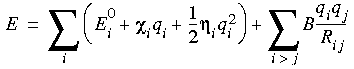 where is the electronegativity and
  the hardness. The first term is just a Taylor series expansion of the energy of each atom as a function of charge, and the second is the Coulomb interaction law between charges. The Coulomb law term introduces a geometry dependence that ESFF for the time being ignores, by considering only topological neighbors at effectively idealized geometries.
Minimizing the energy with respect to the charges leads to the following expression for the charge on atom i:
Eq. 13
 where
where  is the Lagrange multiplier for the constraint on the total charge, which physically is the equalized electronegativity of all the atoms. The
  term contains the geometry-independent remnant of the full Coulomb summation.
Eqns. 12 and 13 give a totally delocalized picture of the charges in a relatively severe approximation. To obtain reasonable charges as judged by, for example, crystal packing calculations, some modifications to the above picture have been made. Metals and their immediate ligands are treated with the above prescription, summing their formal charges to get a net fragment charge. Delocalized  systems are treated in an analogous fashion. And
  systems are treated using a localized approach in which the charges of an atom depend simply on its neighbors. Note that this approach, unlike the straightforward implementations based on the equalization of electronegativity, does include some resonance effects in the system.
Electronegativity and hardness obtained by DFT
The electronegativity and hardness in the above equations must be determined. In earlier forcefields they were often determined from experimental ionization potentials and electron affinities; however, these spectroscopic states do not correspond to the valence states involved in molecules. For this reason, ESFF is based on electronegativities and hardnesses, calculated using density functional theory as implemented in DMol. The orbitals are (fractionally) occupied in ratios appropriate for the desired hybridization state, and calculations are performed on the neutral atom as well as on positive and negative ions.
ESFF uses the 6-9 potential for the van der Waals interactions. Since the van der Waals parameters must be consistent with the charges, they are derived using rules that are consistent with the charges.
Starting with the London formula:
Eq. 14
![]() where is the polarizability and IP the ionization potential of the atoms, the polarizability, in a simple harmonic approximation, is proportional to n / IP where n is the number of electrons. Across any one row of the periodic table, the core electrons remain unchanged, so that the following form is reasonable:
where is the polarizability and IP the ionization potential of the atoms, the polarizability, in a simple harmonic approximation, is proportional to n / IP where n is the number of electrons. Across any one row of the periodic table, the core electrons remain unchanged, so that the following form is reasonable:
Eq. 15
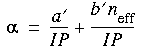 where a´ and b´ are adjustable parameters that should depend on just the period, and neff is the effective number of (valence) electrons. Further assuming that is proportional to R3 and that another equivalent expression to that in Eq. 14 is:
Eq. 16
![]() where
where  is a well depth, the following forms are deduced for the rules for van der Waals parameters:
Eq. 17
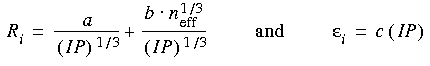 The van der Waals parameters are affected by the charge of the atom.
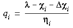
In ESFF we found it sufficient to modify the ionization potential (IP) of metal atoms according to their formal charge and hardness:
Eq. 18
![]() Treatment of nonmetals
Treatment of nonmetals
and for nonmetals to account for the partial charges when calculating the effective number of electrons.
ESFF atom types
ESFF atom types (Table 32) are determined by hybridization, formal charge, and symmetry rules (Atom-typing rules in ESFF). In addition, the rules may involve bond order, ring size, and whether bonds are endo or exo to rings. For metal ligands the cis-trans and axial-equatorial positionings are also considered. The addition of these latter types affects only certain parameters (for example, bond order influences only bond parameters) and thus are not as powerful as complete atom types. In one sense they provide a further refinement of typing beyond atom types.
Coverage of the periodic table
The ESFF forcefield has been parameterized to handle all elements in the periodic table up to radon. It is recommended for organometallic systems and other systems for which other forcefields do not have parameters. ESFF is designed primarily for predicting reasonable structures (both intra- and intermolecular structures and crystals) and should give reasonable structures for organic, biological, organometallic and some ceramic and silicate models. It has been used with some success for studying interactions of molecules with metal surfaces. Predicted intermolecular binding energies should be considered approximate.
UFF, universal forcefield
Cerius2 contains a full implementation of the Universal forcefield, including bond order assignment. The Cerius2 implementation has been rigorously tested and results are in agreement with published work on this forcefield (Rappé et al. 1992, Casewit et al. 1992a, b, Rappé et al. 1993).
UFF is a purely diagonal, harmonic forcefield. Bond stretching is described by a harmonic term, angle bending by a three-term Fourier cosine expansion, and torsions and inversions by cosine-Fourier expansion terms. The van der Waals interactions are described by the Lennard-Jones potential. Electrostatic interactions are described by atomic monopoles and a screened (distance-dependent) Coulombic term.
UFF has full coverage of the periodic table. UFF is moderately accurate for predicting geometries and conformational energy differences of organic molecules, main-group inorganics, and metal complexes. It is recommended for organometallic systems and other systems for which other forcefields do not have parameters.
The Universal forcefield includes a parameter generator that calculates forcefield parameters by combining atomic parameters. Thus, forcefield parameters for any combination of atom types can be generated as required.
-complexation and are associated with explicit parameters.
Important
Charges in the Universal forcefield
The Universal forcefield was developed in conjunction with the charge equilibration (Rappé & Goddard 1991) method. Therefore this method of electrostatic charge calculation is highly recommended for use with the Universal forcefield. For more on the charge equilibration calculation, see the documentation supplied with Cerius2·OFF).
UNIVERSAL1.02 is the most up-to-date, and recommended, version of the UFF. It includes full bond-order correction. (UFF 1.02 differs from UFF 1.01 in that some explicit torsion parameters were corrected and one of the oxygen atom-typing rules was modified.)
VALBOND
Introduction
Most molecular mechanics methods attempt to describe accurate potential energy surfaces by using a variant of the general valence forcefield, and a large number of parameters. These simple forcefields are not accurate outside the proximity of the energetic minima and often are difficult to apply to the different shapes and higher coordination numbers of transition metal complexes.
Validation
Although the original VALBOND was developed for use with the CHARMM forcefield (Brooks et al., 1983), the table below shows that the quality of the new UFF-VALBOND forcefield is comparable to the original, and similar to popular forcefields.
Applicability
UFF-VALBOND can be used for compounds containing elements from across the periodic table.
Assigning VALBOND centers
If the model contains hypervalent atoms, VALBOND centers should be assigned by hand. This may be accomplished as follows:
Cerius2 will assign values for the gross hybridization to VALBOND centers based on the hybridization of the atoms as stored in the data model.
For p-block elements the gross hybridization is of the form spn. For d-block elements VALBOND assumes a hybridization of the form sdm.
In certain cases, i.e., some hypervalent atoms, Cerius2 may not be able to assign a gross hybridization to all atoms, or occasionally, the user may wish to override the assigned values. Gross hybridizations may be assigned manually as follows:
For example the gross hybridization of the N atom in ammonia, NH3, equals three (sp3).
The bond hybridization of the N-H bonds is calculated as sp3.47. The gross hybridization of O in water is three, and the bond hybridization of the O-H bond is sp3.87. Thus VALBOND calculates these bonds to have more p character than the C-H bond in say methane, where both gross and bond hybridizations are sp3, exactly.
Bond hybridizations are calculated when VALBOND centers are assigned.
UFF_VALBOND1.01 via the Open Force Field card.
UFF_VALBOND1.01 via the Open Force Field card.
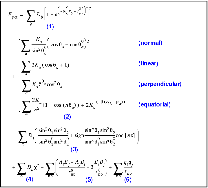
Functional form
The Dreiding forcefield is a purely diagonal forcefield with harmonic valence terms and a cosine-Fourier expansion torsion term. The umbrella functional form is used for inversions, which are defined according to the Wilson out-of-plane definition (see Table 24). The van der Waals interactions are described by the Lennard-Jones potential. Electrostatic interactions are described by atomic monopoles and a screened (distance-dependent) Coulombic term. Hydrogen bonding is described by an explicit Lennard-Jones 12-10 potential (Mayo et al. 1990).
Coverage of the periodic table
The Dreiding forcefield has good coverage for organic, biological and main-group inorganic molecules. It is only moderately accurate for geometries, conformational energies, intermolecular binding energies, and crystal packing.
The Dreiding II forcefield is an extension and improvement over the Dreiding I forcefield. DREIDING2.21 is the recommended, up-to-date version of the Dreiding II forcefield.
Availability
![]()
Classical forcefields
Classical forcefields provided by MSI include AMBER, CHARMm, and CVFF:
The parameters of classical forcefields were derived by fitting experimental data sets. They were generally designed for biological macromolecules, although they have been used or adapted for other classes of models. Since they are relatively old, they are well characterized and many research studies have used them.
AMBER forcefield
The standard AMBER forcefield (Weiner et al. 1984, 1986) is parameterized to small organic constituents of proteins and nucleic acids. Only experimental data were used in parameterization.
AMBER is used mainly for modeling proteins and nucleic acids. It is generally lower in accuracy and has a limited range of applicability. The use of AMBER is recommended mainly for those customers who are familiar with AMBER and have developed their own AMBER-specific parameters. It generally gives reasonable results for gas-phase model geometries, conformational energies, vibrational frequencies, and solvation free energies.
Standard AMBER forcefield
Functional form
The AMBER energy expression contains a minimal number of terms. No cross terms are included. The functional forms of the energy terms used by AMBER are given in Eq. 19.
Eq. 19
 The first three terms in Eq. 19 handle the internal coordinates of bonds, angles, and dihedrals. Term 3 is also used to maintain the correct chirality and tetrahedral nature of sp3 centers in the united-atom representation. (In the united-atom representation, nonpolar hydrogen atoms are not represented explicitly, but are coalesced into the description of the heavy atoms to which they are bonded.) Terms 4 and 5 account for the van der Waals and electrostatic interactions.
The final term, 6, is an optional hydrogen-bond term that augments the electrostatic description of the hydrogen bond. This term adds only about 0.5 kcal mol-1 to the hydrogen-bond energy in AMBER, so the bulk of the hydrogen-bond energy still arises from the dipole-dipole interaction of the donor and acceptor groups.
The atom types in AMBER are quite specific to amino acids and DNA bases. In the original publications, the atom types and charges are defined by means of diagrams of the amino acids and nucleotide bases. In the Insight environment, this information has been placed in a residue library. Descriptions of the atom types, from the original papers defining the AMBER forcefield, are shown in Table 25.
Homans' carbohydrate forcefield
Extension of AMBER to carbohydrates
Homans' forcefield for oligosaccharides (Homans 1990) has been incorporated into the AMBER forcefield available in the Discover program. It uses the same functional form as AMBER and extends its applicability to polysaccharides and glycoproteins.
Homans' approach in developing the carbohydrate forcefield was to combine the parameters for monosaccharides (Ha et al. 1988) with the results of ab initio calculations on model compounds relevant to the glycosidic linkage (Wiberg and Murcko 1989), to generate an AMBER-compatible forcefield. The bond, angle, and torsion parameters for each monosaccharide residue were in general taken directly from Ha et al. (1988). However, certain parameters required adjustment and others were added, to account for the glycosidic linkage between contiguous monosaccharide residues. The torsion parameters were adjusted to fit the quantum mechanical data (6-31G*) of Wiberg and Murcko (1989) for dimethoxymethane.
To account for the anomeric effect associated with carbohydrates, the linking atoms were defined as different atom types. Table 26 lists these atom types, as well as the types corresponding to the ring atoms of sugars.
CHARMm forcefield
CHARMm, which derives from CHARMM (Chemistry at HARvard Macromolecular Mechanics), is a highly flexible molecular mechanics and dynamics program originally developed in the laboratory of Dr. Martin Karplus at Harvard University. It was parameterized on the basis of ab initio energies and geometries of small organic models.
CHARMm performs well over a broad range of calculations and simulations, including calculation of geometries, interaction and conformation energies, local minima, barriers to rotation, time-dependent dynamic behavior, free energy, and vibrational frequencies (Momany & Rone, 1992). CHARMm is designed to give good (but not necessarily "the best") results for a wide variety of modelled systems, from isolated small molecules to solvated complexes of large biological macromolecules; however, it is not applicable to organometallic complexes.
CHARMm uses a flexible and comprehensive empirical energy function that is a summation of many individual energy terms. The energy function is based on separable internal coordinate terms and pairwise nonbond interaction terms (Brooks et al. 1983). The total energy is expressed by the following equation:
Eq. 20
where the oop (out-of-plane) angle is defined as an improper torsion. A more specific (Brooks et al. 1983) statement of the function is:
Eq. 21
 The electrostatic term can be scaled to mimic solvent effects. The van der Waals combination rules and functional form are derived from rare-gas potentials. The function optionally used in CHARMm to calculate the hydrogen bond energy is:
Eq. 22
 Hydrogen bond energy is not included as a default energy term. The current CHARMm parameter set has been derived in such a way that hydrogen bond effects are described by the combination of electrostatic and van der Waals forces.
CVFF, consistent valence forcefield
The consistent-valence forcefield (CVFF), the original forcefield provided with the Discover program (and now available also in Cerius2·OFF), is a generalized valence forcefield (Dauber-Osguthorpe 1988). Parameters are provided for amino acids, water, and a variety of other functional groups.
CVFF was fit to small organic (amides, carboxylic acids, etc.) crystals and gas phase structures. It handles peptides, proteins, and a wide range of organic systems. As the default forcefield in Discover, it has been used extensively for many years. It is primarily intended for studies of structures and binding energies, although it predicts vibrational frequencies and conformational energies reasonably well.
The CDiscover program has undergone extensive validation tests comparing it with FDiscover. These tests have indicated that the two programs provide exactly the same results for all components of the energy expression with one exception: the out-of-plane energy for the CVFF forcefield.
For CVFF, only one of these improper torsions is used. The rules that FDiscover employs to select the particular improper torsion are somewhat arbitrary, and it was not possible to replicate them in CDiscover. However, the changes in energy are very small (on the order of 0.01 kcal mol-1). (A more rigorously defined out-of-plane, the Wilson out-of-plane, is used in the CFF forcefield. This energy term provides exact agreement between CDiscover and FDiscover.)
Functional form
The analytic form of the energy expression used in CVFF is shown in Eq. 23.
Eq. 23
 Types of terms and computational costs
Terms 1-4 are commonly referred to as the diagonal terms of the valence forcefield and represent the energy of deformation of bond lengths, bond angles, torsion angles, and out-of-plane interactions, respectively.
When the model being simulated is high in energy (caused, for example, by overlapping atoms or a high target temperature), a Morse-style function might allow bonded atoms to drift unrealistically far apart (see Figure 2). This would not be desirable unless you were intending to study bond breakage.
|
Terms 5-9 are off-diagonal (or cross) terms and represent couplings between deformations of internal coordinates. For example, Term 5 describes the coupling between stretching of adjacent bonds.
Terms 10-11 describe the nonbond interactions. Term 10 represents the van der Waals interactions with a Lennard-Jones function. Term 11 is the Coulombic representation of electrostatic interactions. The dielectric constant
can be made distance dependent (i.e., a function of rij).
CVFF atom types
The CVFF forcefield supplied by MSI defines atom types for the 20 commonly occurring amino acids, most hydrocarbons, and many other organic models (Table 30).
It automatically supplies generic parameters when specific parameters are not found (Automatic assignment of values for missing parameters).
The augmented version of CVFF (available in version 4.0.0 of the Insight program) includes nonbond parameters (Born model) for additional atom types (Table 31) that are useful for simulations of silicates, aluminosilicates, clays, and aluminophosphates. These added parameters were derived using Ewald summation for nonbond interactions between the additional atom types.
The bond increment section of the .frc file for CVFF has been expanded so that partial charges can be determined whenever the Cerius2·OFF module or the Discover program is able to assign automatic atom types.
Availability
![]()
Special-purpose forcefields
Several forcefields are provided by MSI that are specialized for certain uses:
The specialized forcefields described in the following sections have been developed for the purpose of simulating certain systems or performing limited types of calculationfss well. They should not be used for other purposes, since they were not designed to be accurate outside their limited areas of applicability.
Glass forcefield
The Glass forcefield (Glassff) exists in versions that include two- and three-body nonbond terms (glassff_1.01 and glassff_2.01, respectively) and is used for studying a range of inorganic oxide glasses (and other ionic systems) under periodic boundary conditions. The newer, three-body, glass forcefield is recommended and documented here.
All ion pairs are subjected to an interaction containing a repulsive van der Waals term and a screened Coulombic term.
Eq. 24
 Where:
If you want to customize the glass forcefield, the parameter A for each element combination ij can be computed approximately, using the formula:
 Where:
For models within the scope of the glass forcefield, the default Open Force Field settings included in the file can be used without adjustment. Atom typing and charging also can be done automatically.
MSXX forcefield for polyvinylidene fluoride
The MSXX forcefield for polyvinylidene fluoride (PVDF) and related polymers and small organic models (Karasawa & Goddard 1992) is based on a combination of first-principles quantum mechanical calculations. It includes cross terms (for accurate vibrational frequencies), and charges are associated with each atom type.
Four aspects were addressed to generate an accurate forcefield for PVDF: charges, van der Waals interactions, torsion terms, and valence terms.
Note
|
The MSXX forcefield uses the Morse functional form for bond stretching, which means that the force goes to zero at large bond distances (see Figure 2). Therefore this forcefield should not be used when starting a run with bad initial geometries. Instead, use an alternative forcefield (e.g., the Universal forcefield) when starting from a bad geometry and then switch to the MSXX when close to the energy minimum. |
See also documentation of PCFF (PCFF forcefield for polymers and other materials) and COMPASS (COMPASS forcefield for organic and inorganic materials).
Zeolite forcefields
See also documentation on the augmented CVFF (Augmented CVFF).
The BKS forcefield was developed by van Beest et al. (1990) to describe the geometries, vibrational frequencies, and mechanical properties of silicas and aluminophosphates. The parametrization is based on both ab initio and experimental data. The forcefield contains four atom types: Si, O, Al, and P.
The Burchart forcefield was developed by Burchart (1992) to describe the geometry, heats of formation, transitions under pressure, crystal morphology, and vibrational frequencies of silicas and aluminophosphates. The parametrization is based mainly on experimental data and includes both valence and nonbond terms. It contains four atoms types: Si, O, Al, P.
The Burchart-Universal forcefield combines the Burchart and Universal forcefields. Similar to the Burchart-Dreiding forcefield described above, the Burchart forcefield treats the framework; the Universal forcefield treats the intra- and inter-molecular interactions; and the parameters for the framework-molecule interactions are derived from parameters from both forcefields, combined by the geometric combination rule.
Forcefields for sorption on zeolites
Several forcefields have been implemented especially for studies of sorption of rigid small molecules onto zeolite structures, using the Cerius2·Sorption module. They can be used in studies of binding sites, interaction energies, Henry's constants, adsorption isotherms, and relative selectivity.
The parameters for C, H, O, and Na in the Sorption Yashonath forcefield are taken from Yashonath et al. (1988). Mainly for saturated hydrocarbons in zeolites
The parameters for C, H, O, and Na in the Sorption Demontis forcefield are taken from Demontis et al. (1989). Mainly for benzene in zeolites.
The parameters for O and Xe in the Sorption Pickett forcefield are taken from Pickett et al. (1990). Mainly for xenon in zeolites.
The Watanabe-Austin forcefield (Watanabe et al. 1995) was fit to experimental adsorption isotherms (Miller et al. 1987) for argon, oxygen, and nitrogen adsorption in zeolite types A, X, and Y (alumonosilicates with Ca+2, Na+, and Li+ counterions). It contains parameters for argon, oxygen and nitrogen sorbates, Ca, Na, K, and Li cations, and zeolite framework atoms (Si, Al, O).
Forcefields for Cerius2·Morphology module
These forcefields include only nonbond interaction terms and are intended only for determining crystal morphology in the Cerius2·Morphology module.
In the Morphology/Lifson forcefield (Lifson et al. 1979), you need to assign the charges on the C, C_O, and H_N. Charges should be assigned by assuming electroneutrality of the CH3, CH2, CH, amide, CO, NH, NH2, and COOH groups. This forcefield is recommended for studies of the morphology of crystals or carboxylic acids and amides and is limited to regid-body calculations involving C, H, N, and O.
The Morphology/Williams (Williams 1966) forcefield is applicable only to hydrocarbon crystal morphology, because it contains only parameters for carbon and hydrogen.
The Morphology/Momany and Morphology/Scheraga forcefields (Momany et al. 1974, Némethy et al. 1983) were developed for polypeptides and are suited for predicting the packing configurations and lattice energies in crystals of hydrocarbons, carboxylic acids, amines, and amides (also amino acids and polypeptides for Morphology/Scheraga). They are limited to rigid-body calculations.
Cerius2
![]()
Archived and untested forcefields
Several old and nonvalidated forcefields for the Cerius2·Open Force Field module are included in the untested and archive subdirectories of the forcefield directory (Cerius2-Resources/FORCE-FIELD directory). These forcefields are documented below.
Several of old, nonvalidated, unsupported forcefields for some Insight modules are included in subdirectories of the $BIOSYM/gifts directory. These forcefields are documented (minimally) by means of README files in those directories.
The Cerius2 archive directory contains copies of forcefield files that were previously released with CERIUS, as well as a copy of the Dreiding forcefield previously released with POLYGRAF. Newer versions of most of these forcefields are available in the top-level forcefield directory, as discussed above. These archived forcefields should be used only when necessary for compatibility with work carried out using CERIUS 3.0-3.2 or POLYGRAF.
Most of these are CERIUS forcefields and produce the same results when used in Cerius2 as in CERIUS 3.2. However, GRAFDREIDING1.00 is the Dreiding II forcefield from POLYGRAF3.2.1.
The GRAFDREIDING1.00 forcefield is the direct result of a format conversion (via the pf converter, as discussed in the documentation for C2·OFF) of the dreidii321.par forcefield of POLYGRAF3.2.1. Nevertheless, discrepancies may result between the energies calculated in Cerius2 and in POLYGRAF.
This version of the Dreiding II forcefield also differs from both the published one (Mayo et al. 1990) and the other Dreiding forcefield files in Cerius2 in that this version uses the geometric combination rule for nonbond interactions (see Combination rules for van der Waals terms).
We strongly recommend that you use the UNIVERSAL1.02 or DREIDING2.21 forcefields in preference to the GRAFDREIDING1.00 field, unless you want to match the results of POLYGRAF calculations.
Note
 ij Depends on species.
 0.29 Å.